
In recent years, the demand for high-precision measurement instruments has grown significantly in fields such as lunar exploration, space remote sensing, deep-space exploration, and aerospace. The ability to accurately perceive and measure multi-dimensional force/torque information in space has made six-axis force sensors a focal point in multi-force sensing technology research. These sensors are increasingly applied in military, aerospace, automotive engineering, biomedical, and industrial sectors, offering vast potential. Traditional six-axis force sensors often employ parallel Stewart platform structures or their variants, such as preloaded or flexure-integrated designs, as elastic body configurations. However, existing models typically assume ideal spherical joints and two-force members in measuring branches, neglecting frictional moments and other coupling effects, which limits measurement accuracy. Flexure parallel six-axis force sensors, with their monolithically fabricated flexible joints, provide high motion accuracy, sensitivity, and eliminate the need for repeated calibration, making them suitable for compact spaces. This paper focuses on the flexure parallel Stewart platform six-axis force sensor, proposing an analytical method for precise force mapping between external six-dimensional forces and axial tensions/compressions in flexible measuring branches. The approach is based on the virtual work principle, geometric compatibility conditions, and compliance matrices of flexure hinges, enabling accurate modeling of the sensor’s stiffness and force relationships. The derived analytical model is validated through numerical examples and finite element simulations, demonstrating high accuracy and providing a foundation for dimensional optimization of flexure parallel six-axis force sensors.
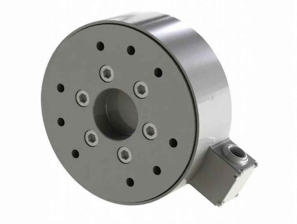
The structure of the flexure parallel six-axis force sensor is illustrated in Figure 1. It consists of a measuring platform connected to a fixed base via six flexible measuring branches. Each branch includes flexure spherical hinges with thin beams at both ends and a flexible branch rod. The centers of the connecting points on the measuring platform, denoted as Oi (i=1,2,…,6), are evenly distributed on a circle of radius R, with points Om (m=1,3,5) and Ok (k=2,4,6) spaced at 120-degree intervals. A reference coordinate system Opxpypzp is fixed at the geometric center of the circle formed by Oi on the lower surface of the measuring platform, with the xp-axis perpendicular upward, the yp-axis along the angular bisector of O1 and O6, and the zp-axis following the right-hand rule. Similarly, a fixed coordinate system Oxyz is established on the upper surface of the fixed base, with the x-axis perpendicular upward and aligned with the xp-axis, the y-axis parallel to yp, and the z-axis following the right-hand rule. The height between the measuring platform and fixed base is H, and the angle θ defines the orientation of O1 relative to the yp-axis.
The flexibility of the sensor arises from the compliance of flexure hinges and branch rods. To model the stiffness, we begin with the compliance matrix of basic flexible elements. For a cantilever beam subjected to six-dimensional loads at its free end, the spatial compliance matrix in its local coordinate system is derived as follows. Consider a cantilever beam with length L, cross-sectional area A, moments of inertia Iy and Iz, elastic modulus E, and shear modulus G. The compliance matrix C for a circular or rectangular cross-section beam is given by:
$$ \mathbf{C} = \begin{bmatrix}
\frac{L}{EA} & 0 & 0 & 0 & 0 & 0 \\
0 & \frac{L^3}{3EI_z} & 0 & 0 & 0 & \frac{L^2}{2EI_z} \\
0 & 0 & \frac{L^3}{3EI_y} & 0 & -\frac{L^2}{2EI_y} & 0 \\
0 & 0 & 0 & \frac{L}{GI_K} & 0 & 0 \\
0 & 0 & -\frac{L^2}{2EI_y} & 0 & \frac{L}{EI_y} & 0 \\
0 & \frac{L^2}{2EI_z} & 0 & 0 & 0 & \frac{L}{EI_z}
\end{bmatrix} $$
where IK is the polar moment of inertia for circular cross-sections or calculated for rectangular cross-sections using:
$$ I_K = bh^3 \left[ \frac{1}{3} – 0.21 \frac{h}{b} \left(1 – \frac{h^4}{12b^4}\right) \right] \quad \text{for} \quad b \geq h $$
For coordinate transformation, the compliance matrix in a reference coordinate system is obtained through a pose transformation matrix. Let Cg be the compliance matrix in the local coordinate system {Og}, and Cpb be the matrix in the reference system {Op}. The transformation is:
$$ \mathbf{C}_{pb} = \mathbf{J}^T \mathbf{C}_g \mathbf{J} $$
where J is the pose transformation matrix from {Og} to {Op}, given by:
$$ \mathbf{J} = \begin{bmatrix}
\mathbf{R} & \mathbf{0} \\
\mathbf{0} & \mathbf{R}
\end{bmatrix} $$
with R being the rotation matrix between the two systems.
Next, we model the compliance of a flexure spherical hinge with thin beams at both ends. The compliance matrix Cps for this component is derived using the virtual work principle and deformation superposition, considering the compliance matrices of the thin beams and the flexure hinge. For a flexure spherical hinge with radius rs, notch spacing t, and beam thicknesses lb1 and lb2, the compliance matrix Cs in its local coordinate system is:
$$ \mathbf{C}_s = \begin{bmatrix}
c_1 & 0 & 0 & 0 & 0 & 0 \\
0 & c_2 & 0 & 0 & 0 & c_3 \\
0 & 0 & c_2 & 0 & -c_3 & 0 \\
0 & 0 & 0 & c_4 & 0 & 0 \\
0 & 0 & -c_3 & 0 & c_5 & 0 \\
0 & c_3 & 0 & 0 & 0 & c_5
\end{bmatrix} $$
where the coefficients c1 to c5 are calculated as:
$$ c_1 = \frac{64 I_1}{\pi E r_s^3}, \quad c_2 = \frac{64 I_2}{\pi E} + \frac{64 \kappa I_3}{\pi G}, \quad c_3 = \frac{64 I_3}{\pi E}, \quad c_4 = \frac{64(1+\nu)I_4}{\pi E}, \quad c_5 = \frac{64 I_5}{\pi E} $$
Here, κ is the shear coefficient (κ=1 for average shear stress), ν is Poisson’s ratio, and I1 to I5 are integrals dependent on the geometry, defined as:
$$ I_1 = \int \frac{1}{\xi(\xi+2)^3} \, d\xi, \quad I_2 = \int \frac{\xi^2 + 6\xi + 10}{(\xi+2)^5} \, d\xi, \quad I_3 = \int \frac{\xi + 4}{(\xi+2)^4} \, d\xi, \quad I_4 = \int \frac{1}{(\xi+2)^2} \, d\xi, \quad I_5 = \int \frac{\xi^2 + 4\xi + 5}{(\xi+2)^4} \, d\xi $$
with ξ = t/(2rs). The overall compliance matrix Cps for the hinge with beams is then:
$$ \mathbf{C}_{ps} = \sum_{j=1}^{3} \mathbf{J}_{sj}^T \mathbf{C}_{sj} \mathbf{J}_{sj} $$
where Jsj are transformation matrices accounting for the positions of the beams and hinge.
For a single flexible serial branch of the six-axis force sensor, which includes two flexure spherical hinges with beams and a flexible branch rod, the compliance matrix at the branch end is derived by combining the compliance matrices of these elements in series. The compliance matrix Cip for the i-th branch is:
$$ \mathbf{C}_{ip} = \sum_{j=1}^{3} \mathbf{J}_{ij}^T \mathbf{C}_{ij} \mathbf{J}_{ij} $$
where Cij are the compliance matrices of the hinges and rod, and Jij are transformation matrices. The stiffness matrix Kip is the inverse of Cip:
$$ \mathbf{K}_{ip} = \mathbf{C}_{ip}^{-1} $$
The overall stiffness matrix K of the six-axis force sensor is obtained by combining the stiffness matrices of all six branches, considering their orientations relative to the reference coordinate system on the measuring platform. Using static equilibrium and geometric compatibility, the overall stiffness matrix is:
$$ \mathbf{K} = \sum_{i=1}^{6} \mathbf{J}_i^{-T} \mathbf{K}_{ip} \mathbf{J}_i^{-1} $$
where Ji are transformation matrices from the local coordinate system of each branch to the reference system. These matrices depend on the spatial distribution of the branches, defined by parameters such as R, θ, and H.
To derive the force mapping relationship, we relate the external six-dimensional force vector F = (fx, fy, fz, mx, my, mz)T applied to the measuring platform to the axial tensions/compressions f = (f1, f2, …, f6)T in the flexible branch rods. The deformation X of the platform under force F is:
$$ \mathbf{X} = \mathbf{C} \mathbf{F} $$
where C = K−1 is the overall compliance matrix. The deformation Xi of the i-th branch end is related to X by:
$$ \mathbf{X}_i = \mathbf{J}_i^{-1} \mathbf{X} $$
The force Fi at the i-th branch end is:
$$ \mathbf{F}_i = \mathbf{K}_{ip} \mathbf{X}_i $$
Using virtual work, the force on the j-th flexible element in the i-th branch is:
$$ \mathbf{F}_{ij} = \mathbf{J}_{ij}^T \mathbf{F}_i $$
Specifically, for the flexible branch rod (j=2), the axial force in its local coordinate system is extracted. Combining for all branches, the force mapping relation is:
$$ \mathbf{f} = \mathbf{G}_{Ff} \mathbf{F} $$
where G_Ff is the force mapping matrix derived as:
$$ \mathbf{G}_{Ff} = \begin{bmatrix}
(\mathbf{J}_{12} \mathbf{J}_{1} \mathbf{K}_{1p} \mathbf{J}_{1}^{-1} \mathbf{C})_{axial} \\
(\mathbf{J}_{22} \mathbf{J}_{2} \mathbf{K}_{2p} \mathbf{J}_{2}^{-1} \mathbf{C})_{axial} \\
\vdots \\
(\mathbf{J}_{62} \mathbf{J}_{6} \mathbf{K}_{6p} \mathbf{J}_{6}^{-1} \mathbf{C})_{axial}
\end{bmatrix} $$
This matrix provides a direct analytical relationship between external forces and internal axial forces, incorporating the compliance of all flexible elements.
For numerical validation, consider a flexure parallel six-axis force sensor with the following parameters: material is beryllium copper (CuBe2) with elastic modulus E = 1.28 GPa, Poisson’s ratio ν = 0.3, and density 8000 kg/m³. The geometric parameters are summarized in Table 1.
| Parameter | Value |
|---|---|
| Radius R | 30 mm |
| Angle θ | 21.68° |
| Length Lf | 8.682 mm |
| Rod length lf | 50.0 mm |
| Hinge radius rs | 4.0 mm |
| Notch spacing t | 1.0 mm |
| Beam thickness lb | 2.0 mm |
The overall stiffness matrix K computed using these parameters is:
$$ \mathbf{K} = 10^{10} \times \begin{bmatrix}
4.1559 & 0 & 0 & 0 & 0 & 0 \\
0 & 42.688 & 0 & 0 & 0 & -1.566 \\
0 & 0 & 42.688 & 0 & 1.566 & 0 \\
0 & 0 & 0 & 0.076 & 0 & 0 \\
0 & 0 & 1.566 & 0 & 1.889 & 0 \\
0 & -1.566 & 0 & 0 & 0 & 1.889
\end{bmatrix} $$
The units are N/m for the top-left 3×3 block, N·m/rad for the bottom-right 3×3 block, and N or N/rad for off-diagonal blocks. The symmetry and low coupling indicate good design isotropy for the six-axis force sensor.
The force mapping matrix G_Ff is calculated as:
$$ \mathbf{G}_{Ff} = \begin{bmatrix}
0.16004 & 0.76011 & -2.10740 & -36.63700 & -5.38840 & -9.33310 \\
0.16004 & -2.20510 & -0.39544 & -36.63700 & -10.77700 & 0.00001 \\
0.16004 & 1.44500 & 1.71200 & -36.63700 & -5.38850 & -9.33310 \\
0.16004 & 1.44500 & -1.71200 & 36.63700 & 5.38850 & 9.33310 \\
0.16004 & -2.20510 & 0.39544 & 36.63700 & 10.77700 & -0.00001 \\
0.16004 & 0.76011 & 2.10740 & 36.63700 & 5.38840 & 9.33310
\end{bmatrix} $$
This matrix allows for the conversion of external forces to axial forces in the branch rods. To validate, finite element analysis (FEA) was performed using Ansys Workbench 14.5. The sensor model was meshed, and various load cases were applied, including uniaxial forces and moments, as well as combined loads. The axial forces in the branch rods were measured from FEA and compared to theoretical values from the force mapping matrix. The results are summarized in Table 2, showing good agreement with errors within 7%, primarily due to minor torsional and bending couplings not fully captured in the model.
| Load Case | f1 (N) | f2 (N) | f3 (N) | f4 (N) | f5 (N) | f6 (N) | Error Range |
|---|---|---|---|---|---|---|---|
| Fx=10 N | 1.600 (T) | 1.600 (T) | 1.600 (T) | 1.600 (T) | 1.600 (T) | 1.600 (T) | 5.39-5.43% |
| 1.692 (S) | 1.692 (S) | 1.692 (S) | 1.692 (S) | 1.692 (S) | 1.692 (S) | ||
| Fy=10 N | 7.603 (T) | -22.055 (T) | 14.452 (T) | 14.452 (T) | -22.055 (T) | 7.603 (T) | 6.10-6.83% |
| 8.158 (S) | -23.550 (S) | 15.390 (S) | 15.392 (S) | -23.554 (S) | 8.161 (S) | ||
| Fz=10 N | -21.078 (T) | -3.954 (T) | 17.124 (T) | -17.124 (T) | 3.954 (T) | 21.078 (T) | 5.25-6.49% |
| -22.476 (S) | -4.173 (S) | 18.309 (S) | -18.311 (S) | 4.175 (S) | 22.483 (S) | ||
| Mx=0.1 N·m | -3.722 (T) | 3.722 (T) | -3.722 (T) | 3.722 (T) | -3.722 (T) | 3.722 (T) | 6.30-6.33% |
| -3.972 (S) | 3.973 (S) | -3.973 (S) | 3.974 (S) | -3.974 (S) | 3.973 (S) | ||
| My=1 N·m | 5.388 (T) | 10.777 (T) | 5.389 (T) | -5.389 (T) | -10.777 (T) | -5.388 (T) | 5.41-5.48% |
| 5.699 (S) | 11.396 (S) | 5.697 (S) | -5.697 (S) | -11.399 (S) | -5.701 (S) | ||
| Mz=1 N·m | -9.333 (T) | 0 (T) | 9.333 (T) | 9.333 (T) | 0 (T) | -9.333 (T) | 5.40-5.47% |
| -9.866 (S) | 0.0024 (S) | 9.871 (S) | 9.873 (S) | 0.0024 (S) | -9.869 (S) | ||
| Combined Load | -15.220 (T) | -26.085 (T) | 33.740 (T) | 2.285 (T) | -14.825 (T) | 29.718 (T) | 3.10-6.52% |
| -16.157 (S) | -27.780 (S) | 35.606 (S) | 2.358 (S) | -15.859 (S) | 31.594 (S) |
In conclusion, this paper presents an analytical method for force mapping in flexure parallel six-axis force sensors. By leveraging compliance matrices of flexible elements and coordinate transformations, we derive the overall stiffness and force mapping relations. The numerical example and FEA validation confirm the accuracy of the approach, with errors within acceptable limits. This methodology provides a foundation for optimizing the design of six-axis force sensors, enhancing their performance in precision applications. The derived force mapping matrix enables direct computation of internal forces from external loads, facilitating sensor calibration and implementation in real-world systems. Future work could focus on dynamic modeling and sensitivity analysis to further improve the six-axis force sensor capabilities.