
In the field of robotics, ensuring safety during human-robot interaction is a critical challenge, particularly for industrial robots operating in shared environments. Traditional approaches often rely on vision sensors or force sensors mounted on the robot’s end-effector to detect collisions, but these methods can be computationally intensive, costly, and less suitable for retrofitting existing industrial systems. To address these limitations, I propose integrating a six-axis force sensor at the robot’s base, which allows for efficient collision detection by compensating for the dynamic forces generated by the robot’s own motion, including gravitational and inertial effects. This article presents a comprehensive dynamic force compensation algorithm that enables the six-axis force sensor to maintain a zero reading during robot movement, thereby facilitating real-time collision detection without external disturbances. The algorithm leverages the Denavit-Hartenberg (D-H) parameter method and Newton-Euler dynamics to model the robot’s structure and compute the forces and moments acting on the base. Through numerical simulations and validation using ADAMS software, I demonstrate the algorithm’s accuracy and applicability, with a focus on a KUKA six-degree-of-freedom robot as a case study. By incorporating multiple formulas and tables, I aim to provide a detailed exposition of the methodology and results, emphasizing the role of the six-axis force sensor in enhancing robotic safety.
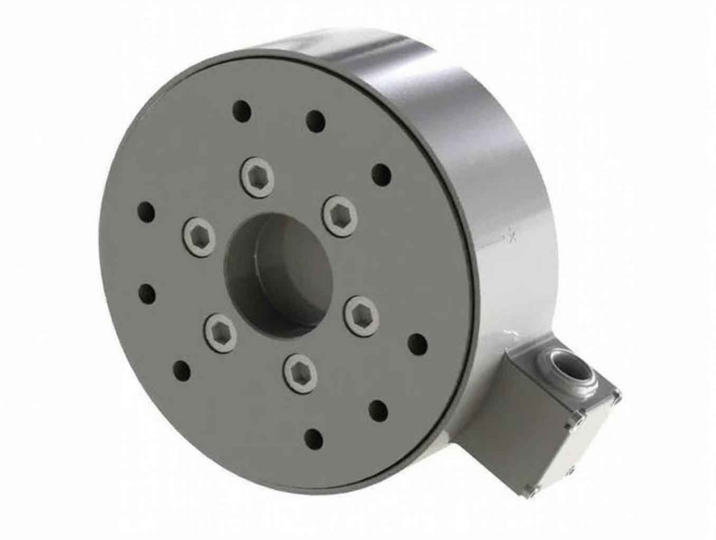
The six-axis force sensor is a versatile device capable of measuring three-dimensional forces and moments, making it ideal for applications requiring force feedback and control. When installed at the robot’s base, it can detect external collisions by isolating the forces attributable to the robot’s own dynamics. However, the robot’s gravitational and inertial forces during movement cause significant variations in the sensor’s zero position, necessitating a dynamic compensation approach. My work builds upon existing gravity compensation techniques but extends them to account for real-time motion effects. The core of the algorithm involves deriving the forces and moments in the sensor coordinate frame through coordinate transformations and dynamic equations, ensuring that the six-axis force sensor readings remain null when no external forces are applied. This not only reduces computational overhead but also improves response times for collision detection in industrial settings.
To model the robot’s kinematics, I employ the D-H parameter method, which defines the relationship between consecutive joint frames. For a robot with n degrees of freedom, the homogeneous transformation matrix from frame {i-1} to frame {i} is given by:
$$^{i-1}_i T = \begin{bmatrix}
\cos \theta_i & -\sin \theta_i \cos \alpha_{i-1} & \sin \theta_i \sin \alpha_{i-1} & a_{i-1} \cos \theta_i \\
\sin \theta_i & \cos \theta_i \cos \alpha_{i-1} & -\cos \theta_i \sin \alpha_{i-1} & a_{i-1} \sin \theta_i \\
0 & \sin \alpha_{i-1} & \cos \alpha_{i-1} & d_i \\
0 & 0 & 0 & 1
\end{bmatrix}$$
where $\theta_i$ is the joint angle, $\alpha_{i-1}$ is the twist angle, $a_{i-1}$ is the link length, and $d_i$ is the link offset. This matrix can be decomposed into a rotation matrix $^{i-1}_i R$ and a position vector $^{i-1}_i p$. The cumulative transformation from the base frame {0} to frame {i} is computed as $^0_i T = ^0_1 T ^1_2 T \cdots ^{i-1}_i T$. For dynamic analysis, the center of mass $c_i$ of link i is defined relative to frame {i} by the vector $c_i = [c_{ix}, c_{iy}, c_{iz}]^T$. The gravitational force vector in the base frame is constant: $G_i = [0, 0, G_i]^T$, where $G_i = m_i g$, with $m_i$ being the mass of link i and g the gravitational acceleration. The gravitational force in the center of mass frame is obtained by rotating the base frame vector: $^{c_i} G_i = ^0_i R^T \cdot ^0 G_i$.
The total force and moment acting on the base due to gravity in the stationary state are derived as follows. The force vector in the base frame is:
$$^0 f = \left[ 0, 0, \sum_{i=1}^n G_i \right]^T$$
and the moment vector is:
$$^0 m = \left[ -\sum_{i=1}^n (G_i \cdot p_{cy,i}), -\sum_{i=1}^n (G_i \cdot p_{cx,i}), 0 \right]^T$$
where $p_{cx,i}$ and $p_{cy,i}$ are the x and y components of the center of mass position in the base frame, computed from $^0_{c_i} T = ^0_i T \cdot ^i_{c_i} T$. To transform these into the sensor frame {S}, which is aligned with the base frame but offset by a distance h along the z-axis, I use the transformation:
$$\begin{bmatrix} ^S f \\ ^S m \end{bmatrix} = \begin{bmatrix} ^S_0 R & 0 \\ ^S(^S p_0) & ^S_0 R \end{bmatrix} \begin{bmatrix} ^0 f \\ ^0 m \end{bmatrix}$$
where $^S_0 R$ is the identity matrix, and $^S(^S p_0)$ is the skew-symmetric matrix derived from the position vector $[0, h, 0]^T$. This provides the gravity compensation values for the six-axis force sensor when the robot is stationary.
For dynamic compensation during motion, I apply the Newton-Euler method, which involves forward and backward recursions to compute velocities, accelerations, and forces. The forward recursion calculates the angular velocity $\omega_i$, angular acceleration $\dot{\omega}_i$, linear acceleration $\dot{v}_i$, and center of mass acceleration $\dot{v}_{c_i}$ for each link i:
$$\omega_{i+1} = ^{i+1}_i R \cdot \omega_i + \dot{\theta}_{i+1} Z_{i+1}$$
$$\dot{\omega}_{i+1} = ^{i+1}_i R \cdot \dot{\omega}_i + ^{i+1}_i R \cdot \omega_i \times \dot{\theta}_{i+1} e_{i+1} + \ddot{\theta}_{i+1} Z_{i+1}$$
$$\dot{v}_{i+1} = ^{i+1}_i R \left[ \dot{v}_i + \dot{\omega}_i \times ^i_{i+1} p + \omega_i \times (\omega_i \times ^i_{i+1} p) \right]$$
$$\dot{v}_{c_{i+1}} = \dot{v}_{i+1} + \dot{\omega}_{i+1} \times r_{i+1} + \omega_{i+1} \times (\omega_{i+1} \times r_{i+1})$$
where $Z_i = [0, 0, 1]^T$, $r_i$ is the vector from joint i to the center of mass, and initial conditions are $\omega_0 = \dot{\omega}_0 = v_0 = \dot{v}_0 = [0, 0, 0]^T$. The backward recursion computes the forces and moments between links, starting from the end-effector. For link i, the Newton and Euler equations are:
$$F_{i-1}^i = F_{i+1}^i + m_i \dot{v}_{c_i} – ^{c_i} G_i$$
$$M_{i-1}^i = M_{i+1}^i – r_{i+1,c_i} \times F_{i+1}^i + r_{i,c_i} \times F_{i-1}^i + I_i \dot{\omega}_i + \omega_i \times (I_i \omega_i)$$
where $F_{i-1}^i$ and $M_{i-1}^i$ are the force and moment exerted by link i-1 on link i, $I_i$ is the inertia tensor of link i about its center of mass, and $r_{i,c_i}$ is the vector from joint i to the center of mass. For a robot with no external load, $F_{n+1}^n = 0$ and $M_{n+1}^n = 0$. The force and moment at the base, $F_0^1$ and $M_0^1$, are then transformed to the sensor frame using the same transformation as in the gravity compensation. The compensated sensor readings are given by:
$$\begin{bmatrix} F \\ M \end{bmatrix} = \begin{bmatrix} D_f – ^S f \\ D_M – ^S m \end{bmatrix} = \begin{bmatrix} 0 \\ 0 \end{bmatrix}$$
where $D_f$ and $D_M$ are the raw sensor readings. This dynamic force compensation algorithm ensures that the six-axis force sensor remains at zero during robot motion, enabling reliable collision detection.
To validate the algorithm, I consider a KUKA KR1000_Titan robot with six degrees of freedom. The D-H parameters for this robot are summarized in Table 1, which defines the kinematic structure for modeling.
| Joint | $\alpha_{i-1}$ (deg) | $a_{i-1}$ (mm) | $\theta_i$ (deg) | $d_i$ (mm) |
|---|---|---|---|---|
| 1 | 0 | 0 | $\theta_1$ | 0 |
| 2 | -90 | 600 | $\theta_2$ | 1100 |
| 3 | 0 | 0 | $\theta_3$ | 1400 |
| 4 | 90 | 65 | $\theta_4$ | 0 |
| 5 | 90 | 0 | $\theta_5$ | 1200 |
| 6 | -90 | 0 | $\theta_6$ | 372 |
Using SolidWorks, I obtain the mass properties, including the mass $m_i$, center of mass position $r_i$, and inertia tensor $I_i$ for each link. For simplicity in numerical computation, I assume no external load and set the velocities of joints 4, 5, and 6 to zero. The joint velocities for joints 1-3 are defined as functions of time to simulate a typical motion profile. The dynamic force compensation values are computed in MATLAB by implementing the D-H transformations and Newton-Euler recursions. The results yield the theoretical forces and moments in the sensor frame, which are plotted over time.
For simulation, I import the robot model into ADAMS, define materials, constraints, and drives corresponding to the joint motions, and set up the six-axis force sensor at the base. The simulation runs for 10 seconds with 500 steps, and the forces and moments in the sensor frame are recorded. Comparing the theoretical curves from MATLAB with the simulation outputs from ADAMS allows me to assess the algorithm’s accuracy. The maximum error in each direction is calculated as:
$$\text{Maximum Error} = \frac{|\text{Theoretical Value} – \text{Simulation Value}|_{\text{max}}}{|\text{Theoretical Value}|_{\text{max}}} \times 100\%$$
The errors for the force and moment components are summarized in Table 2, demonstrating that the algorithm maintains high precision, with the largest error being 4.967% in the z-axis force direction.
| Direction | Force Error (%) | Moment Error (%) |
|---|---|---|
| X-axis | 2.478 | 3.125 |
| Y-axis | 3.842 | 4.213 |
| Z-axis | 4.967 | 3.876 |
The numerical results and simulations confirm the effectiveness of the dynamic force compensation algorithm for the six-axis force sensor. For instance, the forces in the x and y directions show close agreement between theory and simulation, as illustrated by the overlapping curves in the plots. The z-direction forces and moments exhibit higher errors due to the dominant gravitational and inertial components, but they remain within acceptable limits for practical applications. This validation underscores the utility of the six-axis force sensor in real-time collision detection systems, as it can reliably distinguish between internal dynamics and external impacts.
In conclusion, the dynamic force compensation algorithm presented here provides a robust method for maintaining the zero position of a six-axis force sensor mounted at the robot’s base during movement. By integrating kinematic and dynamic modeling, the algorithm accurately compensates for gravitational and inertial forces, enabling efficient collision detection without the need for additional sensors. The case study of the KUKA robot demonstrates the algorithm’s applicability and precision, with errors generally below 5%. This approach is particularly valuable for retrofitting existing industrial robots, as it enhances safety while minimizing computational costs. Future work could explore adaptive compensation for varying payloads and more complex motion trajectories, further leveraging the capabilities of the six-axis force sensor in collaborative robotics.