
In dynamic load environments, noise signals significantly impact the measurement accuracy of six-axis force sensors, which are critical for applications in robotics, aerospace, and industrial automation. These sensors, designed to measure forces and moments along three orthogonal axes, often suffer from internal noise sources such as resistance strain gauges, internal impedance, amplification circuits, and electromagnetic interference. This noise contaminates the original signal during transmission, transformation, and acquisition, leading to reduced precision. To address this, I propose an improved particle filtering algorithm with residual compensation steps (RCPF), specifically applied to the lower E-type membrane of a dual-E elastic body six-axis force sensor. This approach leverages nonlinear system modeling based on the relationship between deflection and strain, and it enhances filtering performance by incorporating residual compensation and stratified resampling techniques. The goal is to maintain real-time performance while improving the accuracy of the six-axis force sensor under dynamic conditions.
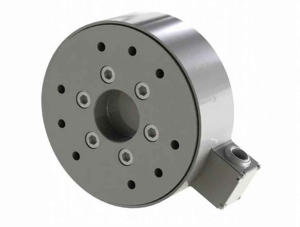
The dual-E elastic body six-axis force sensor comprises an outer force transmission ring, an inner force transmission ring, thin rectangular plates, an upper E-type membrane, a central pillar, a lower E-type membrane, and a base. The upper E-type membrane detects moments in the MX and MY directions, while the lower E-type membrane measures forces in the FX and FY directions (tangential forces) and the FZ direction (normal force). Rectangular beams are used to sense the MZ direction moment. The sensor material is LY12, with an elastic modulus of 72 GPa, a density of 2700 kg/m³, and a Poisson’s ratio of 0.33. This structure allows for precise force and moment detection, but noise remains a challenge in dynamic scenarios.
To model the system, I consider the lower E-type membrane subjected to a normal force FZ, which is transmitted through the central pillar. The mechanical model assumes a fixed outer boundary and an inner boundary under sinusoidal excitation. Based on modal superposition theory and zero initial conditions, the forced vibration deflection function of the E-type membrane can be expressed as an infinite series of principal mode functions and time functions. The deflection \( w(r, \phi, t) \) is given by:
$$ w(r, \phi, t) = \sum_{j=1}^{n} \left[ -\frac{K_j}{\bar{m} (\omega_j^2 – \omega^2)} \frac{\omega}{\omega_j} \sin \omega_j t + \frac{K_j}{\bar{m} (\omega_j^2 – \omega^2)} \sin \omega t \right] W_j(r, \phi) $$
where \( W_j(r, \phi) \) is the principal mode function:
$$ W_j(r, \phi) = [D_{j1} J_n(\lambda r) + D_{j2} Y_n(\lambda r) + D_{j3} I_n(\lambda r) + D_{j4} K_n(\lambda r)] \cos n\phi $$
and \( K_j(r, \phi) \) is the amplitude function:
$$ K_j(r, \phi) = 2\pi K [D’_{j1} J_0(\lambda_j r) + D’_{j2} Y_0(\lambda_j r) + D’_{j3} I_0(\lambda_j r) + D’_{j4} K_0(\lambda_j r)] \cos n\phi $$
Here, \( \omega_j \) is the j-th natural frequency, \( J_n \) and \( Y_n \) are Bessel functions of the first and second kind, \( I_n \) and \( K_n \) are modified Bessel functions, \( \lambda_j = 2\pi \omega_j \sqrt{\frac{\bar{m}}{D}} \) is the natural frequency coefficient, \( \omega \) is the excitation frequency, \( \bar{m} \) is the mass per unit area, and \( D \) is the flexural rigidity. The coefficients \( D_{j1} \) to \( D_{j4} \) and \( D’_{j1} \) to \( D’_{j4} \) are determined from homogeneous linear equations based on boundary conditions.
Using Kirchhoff’s theory for elastic thin plates with small deflections, the radial strain \( \varepsilon(r, \phi, t) \) is derived from the deflection function:
$$ \varepsilon(r, \phi, t) = -\frac{h}{2} \frac{\partial^2 W_j(r, \phi)}{\partial r^2} \sum_{j=1}^{n} \left[ -\frac{K_j}{\bar{m} (\omega_j^2 – \omega^2)} \frac{\omega}{\omega_j} \sin \omega_j t + \frac{K_j}{\bar{m} (\omega_j^2 – \omega^2)} \sin \omega t \right] $$
where \( h \) is the thickness of the circular plate. This leads to a nonlinear discrete-time system model for the six-axis force sensor. The state equation for the strain \( \varepsilon(k) \) at time step \( k \) is:
$$ \varepsilon(k+1) = A e^{a T} \varepsilon(k) + T f(\varepsilon(k), k) – \frac{T p \left( \sum_{j=1}^{i} N_{j,j} \right)}{K} U(k) + T \sum_{j=i+1}^{\infty} \left[ S_j (\cos \omega k – \cos \omega_j k) – f(N_{j,j}) \cdot f(\sin \omega k, k) \right] + T \sum_{j=1}^{i} \left[ S_j (\cos \omega k – \cos \omega_j k) – g(N_{j,j}) \cdot f(\sin n \omega k, k) \right] $$
where \( A \) and \( a \) are convergence coefficients, \( T \) is the sampling period, \( f \) and \( g \) are nonlinear functions, \( N_j = -\frac{h}{2\bar{m}} \frac{K_j}{\omega_j^2 – \omega^2} \frac{\partial^2 W_j(r, \phi)}{\partial r^2} \bigg|_{r=r_x, \phi=\phi_x} \) is the strain gauge centroid coefficient, \( r_x \) and \( \phi_x \) are the centroid position parameters of the strain gauge, and \( U(k) \) is the input force. The measurement equation, based on the Wheatstone bridge principle, relates the output voltage \( Z(k) \) to the strain:
$$ Z(k+1) = f(\varepsilon_{r_x, \phi_x}(k+1)) + V(k+1) $$
where \( V(k+1) \) is Gaussian white noise with zero mean and variance \( R_\sigma \).
Particle filtering is a sequential Monte Carlo method used for state estimation in nonlinear systems. The basic particle filter approximates the posterior probability density \( p(x_k | z_{1:k}) \) using a set of weighted particles \( \{ x_k^i, w_k^i \}_{i=1}^N \). The weights are updated as:
$$ w_k^i = w_{k-1}^i \frac{p(z_k | x_k^i) p(x_k^i | x_{k-1}^i)}{q(x_k^i | x_{k-1}^i, z_k)} $$
where \( q(x_k^i | x_{k-1}^i, z_k) \) is the importance density function. Often, the prior density \( p(x_k^i | x_{k-1}^i) \) is used as the importance function, but it may lead to cumulative errors due to insufficient incorporation of the latest measurements. Resampling is applied to mitigate weight degeneration, but it can cause particle impoverishment, reducing diversity.
To overcome these issues, I developed the RCPF algorithm, which integrates residual compensation and stratified resampling. The steps are as follows:
- Residual Compensation: For each particle \( \tilde{x}_k^i \) at time \( k \), apply residual compensation using:
$$ \tilde{x}_k^i = x_k^i + c_m d_k \mathcal{N}(0, \sigma_k^i) $$
where \( d_k = \frac{(Z_k – f(p(x_k^i | \tilde{x}_{k-1}^{i,\text{best}})))^2}{N} \) is the residual compensation factor, \( c_m \geq 1 \) is a weakening factor, and \( \sigma_k^i \) is the variance of the process noise \( W(k) \). This step incorporates the latest observation \( Z_k \) to correct the prior distribution error. - Stratification: If the effective sample size \( N_{\text{eff}} \) falls below a threshold \( N_{\text{th}} \), partition the particle set \( \{ \tilde{x}_k^i \}_{i=1}^N \) into three subsets based on weight degeneration thresholds \( \alpha \) and \( \beta \):
- High-weight subset \( W_H = \{ \tilde{x}_k^i \}_{i=1}^M \)
- Medium-weight subset \( W_M = \{ \tilde{x}_k^i \}_{i=1}^{N-M-Q} \)
- Low-weight subset \( W_D = \{ \tilde{x}_k^i \}_{i=1}^Q \)
- Thompson-Taylor Aggregation Resampling: Combine particles from \( W_H \) and \( W_D \) to generate a new medium-weight set:
- Compute the weighted aggregate center \( \bar{x}_k \):
$$ \bar{x}_k = \sum_{i=1}^N \tilde{x}_k^i w_k^i $$ - Generate uniformly distributed random numbers \( \{ u_i \}_{i=1}^m \sim U\left( \frac{1}{m} – \frac{\sqrt{3m – 3}}{m^2}, \frac{1}{m} + \frac{\sqrt{3m – 3}}{m^2} \right) \), where \( m = M + Q \).
- Adjust particles using:
$$ \tilde{x}_k^{‘i} = \bar{x}_k + u_i (\tilde{x}_k^i – \bar{x}_k) \quad \text{for } i = 1, 2, \ldots, M+Q $$
- Compute the weighted aggregate center \( \bar{x}_k \):
- Fusion: Merge the optimized set \( \{ \tilde{x}_k^i \}_{i=1}^{N-Q-M} \) with \( \{ \tilde{x}_k^{‘i} \}_{i=1}^{M+Q} \) to form the resampled particle set \( S = \{ \tilde{x}_k^{i,\text{best}} \}_{i=1}^N \), and normalize the weights.
The computational complexity of RCPF is \( O(N) \), similar to basic particle filters, ensuring real-time feasibility for the six-axis force sensor. The complexity is given by:
$$ C(N, M, Q) = N(c_1 + c_2 + c_3 + c_4) + (M + Q)(c_5 + c_6 + c_7) $$
where \( c_1 \) to \( c_7 \) represent computation costs for residual factor calculation, particle compensation, threshold comparisons, aggregation, random number generation, and particle adjustment.
For experimental validation, I applied RCPF to a dynamic test system of the six-axis force sensor. The system includes a data analysis PC, a dynamic calibration platform, a virtual instrument NI-PXI-1042Q, a controller PXI-8196, a board PXI-4461, amplification circuits, and a piezoelectric ceramic drive module. The six-axis force sensor is fixed on the platform, and a sinusoidal excitation force \( P(t) = 20 \sin(200t) \) is applied in the FZ direction. The output signals are amplified and acquired by the data acquisition module.
To simplify the model, I considered a second-order system for the lower E-type membrane. The state equation reduces to:
$$ \varepsilon(k+1) = 0.0526 \varepsilon(k) + 0.025 \varepsilon^2(k) – 8.4547 \times 10^{-3} \cos(200k) – 8.7303 \times 10^{-3} \cos(666k) + 2.7566 \times 10^{-4} \cos(5362k) + W(k) $$
where \( W(k) \) is Gaussian white noise with zero mean and variance 0.001. The measurement equation is:
$$ Z(k+1) = \frac{-14.5046 \varepsilon(k+1)}{100 + 6.8613 \varepsilon(k+1)} + V(k+1) $$
with \( V(k+1) \) having variance \( R_\sigma \). Parameters include inner radius 50 mm, outer radius 100 mm, thickness \( h = 2 \) mm, strain gauge positions \( r_{x1} = r_{x4} = 40 \) mm, \( r_{x2} = r_{x3} = 20 \) mm, \( \phi_{x1} = \phi_{x2} = \pi/4 \), \( \phi_{x3} = \phi_{x4} = 5\pi/4 \), strain gauge sensitivity \( K_s = 1.4 \), initial resistance \( R = 50 \Omega \), and amplitude ratio \( c = 3.9009 \). Natural frequency coefficients are \( \lambda_1 = 99.3966 \) and \( \lambda_2 = 184.6480 \).
I conducted Monte Carlo simulations with 50 time steps, using \( N = 500 \) particles and \( c_m = 1.2 \). The RCPF algorithm was compared against partial resampling particle filter (PRPF) and extended Kalman particle filter (EKPF). The state estimation curves and absolute error curves demonstrate that RCPF provides closer estimates to the true values, with smaller errors. The mean squared error (MSE) and computation time are summarized in the table below:
| Algorithm | Particle Number | MSE | Computation Time (s) |
|---|---|---|---|
| PRPF | 500 | 0.0043228 | 0.4381 |
| EKPF | 500 | 0.0039074 | 0.6447 |
| RCPF | 500 | 0.0011975 | 0.4915 |
The results show that RCPF achieves lower MSE than PRPF and EKPF, with computation time comparable to PRPF and lower than EKPF. This indicates that RCPF enhances estimation accuracy while maintaining real-time performance for the six-axis force sensor.
In conclusion, the RCPF algorithm effectively addresses particle degeneration and impoverishment in nonlinear filtering for six-axis force sensors. By integrating residual compensation and stratified resampling, it improves particle diversity and estimation precision. The application to the lower E-type membrane demonstrates significant performance gains in dynamic environments, ensuring high accuracy and real-time operation for the six-axis force sensor. Future work could explore structural anomaly detection and adaptive parameter tuning to further optimize the algorithm.