
In recent years, electrically driven quadruped robots have demonstrated impressive dynamic locomotion capabilities, enabling them to traverse complex terrains and perform various tasks. However, a significant challenge hindering their prolonged operation is thermal management. During high-load activities, joint motors in these robot dogs can overheat, triggering automatic shutdowns to prevent damage. This reactive protection mechanism limits the robot’s operational time and reliability. To address this, effective thermal management systems are essential, requiring accurate prediction of motor temperatures across the entire quadruped robot. Existing thermal models often focus on individual motors, neglecting the complex heat exchange in compact designs where multiple heat sources, such as motors and onboard computers, interact closely. This oversight reduces prediction accuracy. In this work, we propose a whole-body thermal model based on the lumped-parameter thermal network (LPTN) method, which comprehensively accounts for self-heating, inter-motor heat conduction, heat exchange with onboard computers, joint friction, and forced convection during movement. By identifying model parameters using the least squares method, we achieve precise temperature distribution predictions under various speeds, gaits, and load conditions. Our approach significantly improves accuracy compared to single-motor models, with maximum errors below 5°C, and enables applications in simulation integration, fault detection, and operational time prediction.
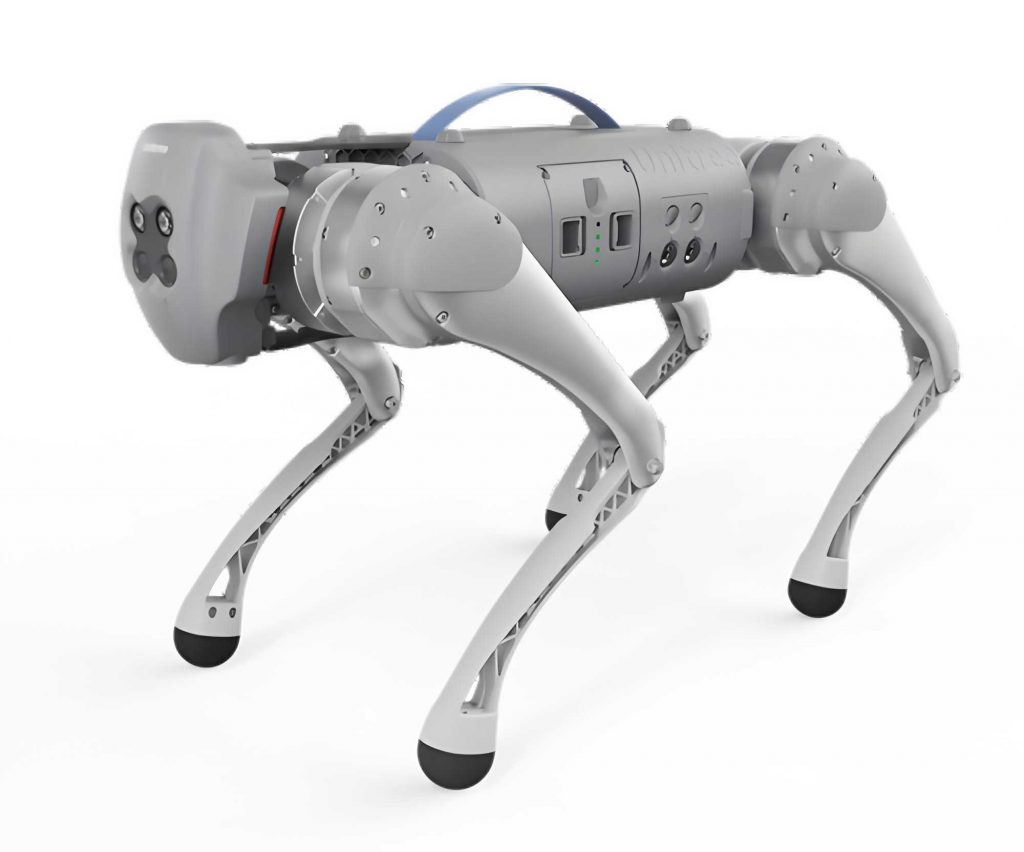
Quadruped robots, often referred to as robot dogs, typically incorporate 12 permanent magnet synchronous motors driven by field-oriented control (FOC) without active cooling systems. In compact designs, motors are densely packed, leading to significant thermal coupling effects. For instance, in many commercial quadruped robots like the Unitree A1, knee joint motors are positioned near hip joint motors, facilitating heat exchange. Additionally, onboard computers for motion control and perception generate substantial heat, further influencing motor temperatures. Traditional single-node motor thermal models, which consider only a motor’s self-heating and natural convection to the environment, fail to capture these interactions, resulting in underestimated temperatures in coupled regions. Our whole-body thermal model addresses this by modeling the entire robot as a network of thermal nodes, each representing a motor or heat source, connected by thermal resistances that emulate heat conduction and convection paths.
The foundation of our thermal modeling begins with a single-node motor thermal model, which simplifies a motor into one node representing the winding and casing in thermal equilibrium. The heat input $Q_{\text{in}}$ is primarily due to copper losses and additional sources like drive electronics:
$$Q_{\text{in}} = I^2 R_d + Q_{\text{other}}$$
where $I$ is the motor current, $R_d$ is the winding resistance, and $Q_{\text{other}}$ includes constant heat from drives and friction. The temperature change is governed by:
$$\frac{dT}{dt} = \frac{Q_{\text{in}} – (T – T_E) / R_{M \sim E}}{C_M}$$
Here, $T$ is the motor temperature, $T_E$ is the ambient temperature, $C_M$ is the thermal capacitance, and $R_{M \sim E}$ is the thermal resistance to the environment, modeled to account for natural and forced convection:
$$R_{M \sim E} = R_c e^{-\beta (T – T_E)} / (1 + \gamma |V_{xy}|)$$
where $R_c$ is conduction resistance, $\beta$ is the natural convection coefficient, $\gamma$ is the forced convection coefficient, and $V_{xy}$ is the robot’s horizontal velocity. This single-node model, while useful for isolated motors, lacks accuracy in multi-motor systems due to ignored thermal couplings.
To capture leg-level interactions, we extend the model to a single-leg thermal network. For a leg with three joints (abduction/adduction, hip flexion/extension, and knee flexion/extension), we define nodes $N_0$, $N_1$, and $N_2$ for each joint motor, connected by thermal resistances $R_{0 \sim 1}$, $R_{1 \sim 2}$, and $R_{0 \sim 2}$ to account for direct and indirect heat paths. Each node has a thermal capacitance $C_i$ and heat input $Q_i$. The temperature dynamics for node $i$ are given by:
$$\frac{dT_i}{dt} = \frac{q_i}{C_i}$$
where the heat flow $q_i$ is:
$$q_i = \sum_{j \in M(i)} \frac{T_i – T_j}{R_{i \sim j}} + I_i^2 R_{i,d} + Q_{i,\text{other}}$$
$M(i)$ denotes the set of nodes connected to $i$, $R_{i,d}$ is the resistance (temperature-dependent as $R_{i,d} = [1 + \alpha_i (T – T_{\text{ref}})] R_{i,d,\text{ref}}$), and $Q_{i,\text{other}}$ includes friction heat from joint movements, modeled using a Coulomb-viscous friction model:
$$F(\dot{q}_i) = -F_{i,k} \cdot \text{sgn}(\dot{q}_i) – D_i \dot{q}_i$$
with $F(\dot{q}_i)$ as the friction torque, $\dot{q}_i$ as the joint velocity, $F_{i,k}$ as the Coulomb friction, and $D_i$ as the damping coefficient. The friction heat over time $\Delta t$ is:
$$Q_{i,\text{friction}} = -F(\dot{q}_i) \int_t^{t+\Delta t} |\dot{q}_i| dt$$
This single-leg model improves accuracy but still omits inter-leg and computer interactions.
For the whole-body thermal model of the quadruped robot, we define 12 motor nodes (e.g., $N_{10}$ for left front abduction, $N_{11}$ for left front hip, $N_{12}$ for left front knee) and one node for the onboard computer ($N_{\text{PC}}$). Thermal resistances connect adjacent motors and the computer, as shown in the network diagram. The state-space representation is:
$$\dot{x} = A x + B u$$
$$y = C x$$
where $x$ is the temperature vector, $u$ is the input vector (copper losses and other heat sources), $A$ is the state matrix encoding thermal resistances, $B$ is the input matrix, and $C$ is the output matrix (identity for direct temperature measurement). To implement this numerically, we discretize the model using a zero-order hold with sampling interval $h$:
$$x(k+1) = G(h) x(k) + H(h) u(k)$$
$$y(k) = C x(k)$$
with approximations $G(h) \approx h A + I$ and $H(h) \approx h B$ for small $h$.
Parameter identification is crucial for model accuracy. We collect data from the robot dog under various conditions, including different torque commands, gaits (trotting, walking), and loads, as summarized in Table 1. The least squares method minimizes the cost function:
$$L(\theta) = \sum_{k=1}^n (x_k – \hat{x}_k)^T (x_k – \hat{x}_k)$$
where $\theta$ represents parameters like thermal resistances, capacitances, and convection coefficients. To balance data from motors with varying torque levels, we apply weighting. A regularization term is added to penalize differences between left and right leg parameters:
$$J(\theta) = L(\theta) + \lambda \sum_{m=1,3} \sum_{n=0}^2 \left( \frac{R_{mn,d}}{C_{mn}} – \frac{R_{(m+1)n,d}}{C_{(m+1)n}} \right)^2$$
Optimization yields $\theta^* = \arg \min_\theta J(\theta)$. Discretization with $h=1$ s uses averaged temperature and root-mean-square torque over intervals.
| Robot State | Torque (N·m) |
|---|---|
| All joints unpowered | 0 |
| Natural cooling | 0 |
| Right front, left rear abduction joints powered | 2/4/6 |
| Right front, left rear hip joints powered | 2/4/6 |
| Right front, left rear knee joints powered | 2/4/6/10 |
| Left front, right rear abduction joints powered | 2/4/6 |
| Left front, right rear hip joints powered | 2/4/6 |
| Left front, right rear knee joints powered | 2/4/6/10 |
| Low-speed trot (max $V_{xy} = 0.2$ m/s) | – |
| Medium-speed trot (max $V_{xy} = 0.5$ m/s) | – |
| High-speed trot (max $V_{xy} = 1.0$ m/s) | – |
Experiments on a Unitree A1 quadruped robot validate our model. We measure joint temperatures, velocities, and torques at 100 Hz, alongside ambient temperature. Identification results show that the whole-body model reduces average fitting errors significantly compared to the single-node model, as seen in Table 2. For instance, the whole-body model’s average error across all joints is 0.74°C, versus 2.02°C for the single-node model.
| Joint Type | Single-Node Model Error (°C) | Whole-Body Model Error (°C) |
|---|---|---|
| Abduction Joint | 1.57 | 0.67 |
| Hip Joint | 2.07 | 0.66 |
| Knee Joint | 2.44 | 0.88 |
| All Joints | 2.02 | 0.74 |
Testing under diverse conditions—standing, trotting with 0 kg and 4 kg loads, and walking—reveals that the whole-body model maintains errors below 5°C, with maximum error reduction over 29% and mean square error reduction over 25% compared to the single-node model. For example, in a high-speed trot, the whole-body model’s maximum error is 2.38°C, while the single-node model reaches 7.11°C. Thermal coupling effects are evident: when one joint is powered, adjacent joints show temperature rises that the single-node model misses. Similarly, forced convection during movement reduces temperature rise rates, which the whole-body model captures through velocity-dependent thermal resistance.
We further evaluate the whole-body model in multi-gait, variable-load scenarios. The robot executes a sequence of tasks: unloaded standing, loaded standing, trotting with 2 kg and 4 kg loads, and walking with 4 kg load. Temperature predictions for all 12 joints closely match measurements, with maximum errors around 3.34°C in the left front knee joint. Table 3 summarizes key results, highlighting the model’s robustness.
| Test Condition | Max Error (°C) | Mean Square Error (°C²) | Error Reduction (%) |
|---|---|---|---|
| Identification Data | 4.77 | 0.91 | 66.67 |
| Standing Still | 2.56 | 0.50 | 51.41 |
| 0 kg Load, Low-Speed Trot | 3.20 | 1.07 | 69.31 |
| 0 kg Load, High-Speed Trot | 2.38 | 0.61 | 66.67 |
| 4 kg Load, Low-Speed Trot | 4.52 | 1.91 | 40.26 |
| 4 kg Load, Walking Gait | 3.47 | 1.14 | 29.44 |
| Natural Cooling | 3.14 | 2.14 | 37.88 |
The whole-body thermal model enables several practical applications. First, integration into robot simulation environments like Gazebo provides real-time temperature predictions during virtual experiments. By feeding joint forces, velocities, and body speeds into the model, we output temperatures for display on simulated joints. In tests, simulated temperatures align closely with real robot data, facilitating controller development with thermal constraints.
Second, the model serves as redundant information for fault detection in motor temperature sensors. If a sensor fails or drifts, the predicted temperature can trigger alerts when deviations exceed a threshold (e.g., 10°C). In simulations, we emulate sensor aging by adding linear errors; the model successfully flags faults when discrepancies arise, enhancing safety for the quadruped robot.
Third, we predict the time until motors reach critical temperatures (e.g., 60°C) under current operating conditions. By extrapolating recent joint states (e.g., 10 gait cycles) into the future using the model, we estimate remaining operation time. For instance, in a 4 kg trot, the knee joint reaches the threshold in approximately 553 seconds. This predictive capability aids in planning and autonomy for robot dogs.
In conclusion, our whole-body thermal model based on lumped-parameter thermal networks effectively addresses the limitations of single-motor models in quadruped robots. By incorporating thermal couplings, convection effects, and multiple heat sources, we achieve accurate temperature predictions with errors under 5°C across varied scenarios. This model not only improves thermal management but also enables advanced applications in simulation, fault detection, and operational forecasting. Future work will focus on enhancing model precision with additional sensors and environmental factors, and integrating it into reinforcement learning for adaptive thermal control in quadruped robots.