
In recent years, the field of robotics has seen significant advancements, with legged robots, particularly quadruped robots, gaining attention due to their superior adaptability to complex terrains. These robot dogs mimic biological locomotion, offering enhanced mobility and efficiency. However, challenges such as limited obstacle avoidance capabilities and energy inefficiencies persist, often stemming from suboptimal leg mechanism designs. This paper addresses these issues by innovatively designing an eight-bar leg mechanism for a quadruped robot, optimizing its dimensions to maximize foot workspace and minimize energy consumption. We employ genetic algorithms for multi-objective optimization, supported by kinematic and dynamic modeling, and validate our approach through simulations. The results demonstrate substantial improvements in performance, providing a robust framework for developing high-performance quadruped robots.
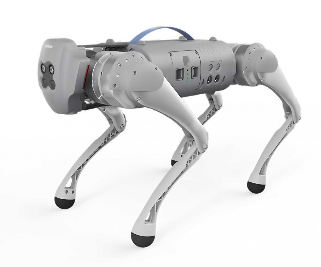
The design of the quadruped robot’s leg mechanism draws inspiration from the skeletal structure of horses, known for their exceptional mobility and obstacle negotiation. By analyzing the equine hindlimb, we derived an open-chain configuration and transformed it into a closed-chain eight-bar mechanism to reduce inertial effects and actuator loads. This transformation ensures consistency in degrees of freedom and workspace equivalence. The robot dog leg consists of key joints such as the hip, knee, and ankle, driven by a combination of rotary actuators and a linear system. The initial parameters, based on biological data, include segment lengths and drive angles, which are parameterized for further analysis. The overall quadruped robot structure comprises a frame, power source, control unit, and four identical legs, each featuring a hybrid serial-parallel arrangement to balance flexibility and efficiency.
To establish a theoretical foundation, we developed kinematic and dynamic models for the eight-bar leg mechanism. The kinematic analysis involves solving closed-loop vector equations for the five-bar subsystems. For the first five-bar mechanism OACEB, the vector balance equation is given by:
$$ \vec{L}_{OA} + \vec{L}_{AC} + \vec{L}_{CE} = \vec{L}_{OB} + \vec{L}_{BE} $$
This translates to the following scalar equations:
$$ -L_1 + L_3 \cos \theta_1 + L_6 \cos \theta_4 = L_2 \cos \theta_2 + L_{45} \cos \theta_3 $$
$$ L_3 \sin \theta_1 + L_6 \sin \theta_4 = L_2 \sin \theta_2 + L_{45} \sin \theta_3 $$
Simplifying, we obtain:
$$ M \sin \theta_2 + N \cos \theta_2 = P $$
where:
$$ M = -2L_2 L_3 \sin \theta_1 – 2L_2 L_6 \sin \theta_4 $$
$$ N = 2L_1 L_2 – 2L_2 L_3 \cos \theta_1 – 2L_2 L_6 \cos \theta_4 $$
$$ P = -(L_2^2 + L_1^2 + L_3^2 + L_6^2 – L_{45}^2 + 2L_3 L_6 \cos \theta_1 \cos \theta_4 + 2L_3 L_6 \sin \theta_1 \sin \theta_4 – 2L_1 L_3 \cos \theta_1 – 2L_1 L_6 \cos \theta_4) $$
Using the tangent half-angle substitution, the solution for $\theta_2$ is:
$$ \theta_2 = 2 \arctan \left( \frac{M + \sqrt{M^2 + N^2 – P^2}}{N + P} \right) $$
Similarly, $\theta_3$ is derived as:
$$ \theta_3 = 2 \arctan \left( \frac{M_2 – \sqrt{M_2^2 + N_2^2 – P_2^2}}{N_2 + P_2} \right) $$
with:
$$ M_2 = -2L_3 L_{45} \sin \theta_1 – 2L_6 L_{45} \sin \theta_4 $$
$$ N_2 = 2L_1 L_{45} – 2L_3 L_{45} \cos \theta_1 – 2L_6 L_{45} \cos \theta_4 $$
$$ P_2 = -2L_3 L_6 \cos \theta_1 \cos \theta_4 – 2L_3 L_6 \sin \theta_1 \sin \theta_4 + L_2^2 – L_1^2 – L_3^2 – L_6^2 – L_{45}^2 + 2L_1 L_3 \cos \theta_1 + 2L_1 L_6 \cos \theta_4 $$
For the second five-bar mechanism EDPQGF, the vector equation is:
$$ \vec{L}_{ED} + \vec{L}_{DP} + \vec{L}_{PQ} + \vec{L}_{QG} = \vec{L}_{EF} + \vec{L}_{FG} $$
Solving for the linear actuator length $L_{10}$:
$$ L_{10} = \sqrt{M_3^2 + N_3^2} $$
where:
$$ M_3 = L_7 \cos \theta_{13} + L_8 \cos \theta_5 – (L_5 \cos \theta_{10} + L_{DP} \cos \theta_{11} + L_{QG} \cos \theta_{12}) $$
$$ N_3 = L_7 \sin \theta_{13} + L_8 \sin \theta_5 + L_5 \sin \theta_{10} – L_{DP} \sin \theta_{11} – L_{10} \sin \theta_8 – L_{QG} \sin \theta_{12} $$
Dynamic modeling employs the Lagrangian method to compute joint torques. The Lagrangian function $L$ is defined as:
$$ L(\theta, \dot{\theta}) = T(\theta, \dot{\theta}) – U(\theta, \dot{\theta}) $$
where $T$ is the total kinetic energy and $U$ is the total potential energy. The kinetic energy for each link is:
$$ T = \sum_{i=1}^{n} \frac{1}{2} (m_i v_i^2 + I_i \dot{\theta}_i^2) $$
and the potential energy is:
$$ U = \sum_{i=1}^{n} m_i g h_i $$
The joint torques $\tau_1$, $\tau_2$, and $\tau_5$ are derived as:
$$ \tau_1 = \frac{d}{dt} \frac{\partial T}{\partial \dot{\theta}_1} – \frac{\partial T}{\partial \theta_1} + \frac{\partial U}{\partial \theta_1} $$
$$ \tau_2 = \frac{d}{dt} \frac{\partial T}{\partial \dot{\theta}_2} – \frac{\partial T}{\partial \theta_2} + \frac{\partial U}{\partial \theta_2} $$
$$ \tau_5 = \frac{d}{dt} \frac{\partial T}{\partial \dot{\theta}_5} – \frac{\partial T}{\partial \theta_5} + \frac{\partial U}{\partial \theta_5} $$
To validate the models, we conducted simulations using ADAMS software. The foot trajectory and joint torques from simulations closely matched the theoretical calculations, confirming model accuracy. For instance, the foot-end trajectory displayed smooth and continuous paths, and torque profiles showed consistent trends, with minor deviations due to friction effects.
For optimization, we focused on two objectives: maximizing the foot workspace and minimizing energy consumption per cycle. The foot workspace area is calculated using the Monte Carlo method, which estimates the area by randomly sampling foot positions. The energy consumption is defined as the sum of absolute joint torques over a cycle:
$$ \text{Minimize} \quad E = \sum_{i=1}^{n} (|\tau_{1i}| + |\tau_{2i}| + |\tau_{5i}|) $$
In single-objective optimization for workspace, we constrained the leg segment lengths $L_3$, $L_{67}$, and $L_{89}$ to sum to 1, with bounds to avoid extreme proportions. The constraints are:
$$ 0.2 \leq L_3 \leq 0.4 $$
$$ 0.2 \leq L_{67} \leq 1 – L_3 – 0.1 $$
$$ 0.2 \leq L_{89} \leq 1 – L_3 – L_{67} $$
$$ L_3 + L_{67} + L_{89} = 1 $$
We evaluated nine combinations, and the results are summarized in the table below:
| Combination | $L_3$ | $L_{67}$ | $L_{89}$ | Workspace Area (m²) |
|---|---|---|---|---|
| 0 | 0.31 | 0.38 | 0.31 | 0.1243 |
| 1 | 0.2 | 0.2 | 0.6 | 0.1266 |
| 2 | 0.2 | 0.3 | 0.5 | 0.1281 |
| 3 | 0.2 | 0.4 | 0.4 | 0.1234 |
| 4 | 0.3 | 0.2 | 0.5 | 0.1301 |
| 5 | 0.3 | 0.3 | 0.4 | 0.1267 |
| 6 | 0.3 | 0.4 | 0.3 | 0.1230 |
| 7 | 0.4 | 0.2 | 0.4 | 0.1248 |
| 8 | 0.4 | 0.3 | 0.3 | 0.1239 |
| 9 | 0.4 | 0.4 | 0.2 | 0.1187 |
Combination 4 yielded the largest workspace area of 0.1301 m², a 4.7% increase over the biological baseline. This highlights the importance of the knee segment proportion in enhancing the robot dog’s mobility.
For energy optimization, we used a genetic algorithm to optimize the lengths $L_1$, $L_2$, $L_3$, $L_{45}$, $L_6$, $L_{67}$, and $L_{89}$. The algorithm parameters were set as follows:
| Parameter | Value |
|---|---|
| Population Size | 50 |
| Maximum Generations | 200 |
| Crossover Probability | 0.8 |
| Pareto Fraction | 0.35 |
| Function Tolerance | 10^{-4} |
| Stall Generations | 20 |
The optimized leg segment lengths reduced the energy consumption from 2059.3 N·m to 1374 N·m, a 33.27% decrease. The comparison of joint torques before and after optimization shows significant reductions in $\tau_1$ and $\tau_2$, while $\tau_5$ remained relatively stable due to the linear actuator design.
In multi-objective optimization, we combined both goals using a weighted sum approach. The Pareto front was generated to explore trade-offs. The optimized dimensions are:
| Parameter | Original Length (mm) | Optimized Length (mm) |
|---|---|---|
| $L_1$ | 400 | 441 |
| $L_2$ | 320 | 370 |
| $L_3$ | 360 | 400 |
| $L_{45}$ | 518 | 628 |
| $L_6$ | 151 | 185 |
| $L_{67}$ | 434 | 273 |
| $L_{89}$ | 353 | 426.5 |
After optimization, the foot workspace area increased to 0.12712 m² (a 2.30% improvement), and energy consumption decreased to 1631.45 N·m (a 20.78% reduction). This demonstrates the effectiveness of the multi-objective approach in balancing performance and efficiency for the quadruped robot.
The genetic algorithm efficiently explored the design space, converging to solutions that enhance both workspace and energy metrics. The knee segment length $L_{67}$ played a critical role, as shorter lengths reduced inertia and torque requirements. Additionally, the hip and ankle segments were adjusted to maintain kinematic consistency. The optimized quadruped robot leg mechanism shows promise for applications in rough terrain navigation, where large workspace and low energy consumption are crucial. Future work will involve physical prototyping and experimental validation to further refine the design.
In conclusion, this study presents a comprehensive framework for designing and optimizing an eight-bar leg mechanism for quadruped robots. By integrating biomechanical inspiration, precise modeling, and advanced optimization techniques, we achieved significant improvements in the robot dog’s performance. The genetic algorithm-based approach provides a scalable method for tailoring leg designs to specific tasks, contributing to the development of more agile and efficient quadruped robots. The results underscore the importance of dimensional optimization in overcoming the limitations of traditional leg mechanisms, paving the way for next-generation autonomous systems.