
Abstract This paper presents a comprehensive study on the biomimetic structural design and gait optimization of a hexapod robot, inspired by the locomotion mechanics of spiders. By integrating bionic principles with advanced robot technology, we address the stability challenges of traditional hexapod robots through innovative leg design and trajectory planning. A novel foot trajectory based on 11th-order Bézier curves is proposed and validated through comparative experiments with the traditional composite cycloid method. The results demonstrate significant improvements in motion stability, highlighting the potential of this approach for advancing robot technology in autonomous navigation and complex terrain adaptation.
Keywords: hexapod robot; biomimetic design; robot technology; Bézier curves; gait optimization
1. Introduction
The field of robot technology has witnessed remarkable advancements in recent years, particularly in the development of legged robots for diverse applications such as search-and-rescue, space exploration, and industrial inspection. Hexapod robots, with their inherent stability due to multi-point support, have emerged as a promising subclass. However, existing designs often suffer from suboptimal structural configurations and foot trajectory planning, leading to instability during movement .
In nature, spiders exhibit exceptional mobility and stability on various terrains, thanks to their six-legged architecture and sophisticated joint mechanics. Leveraging these biological insights, this study aims to enhance hexapod robot performance through biomimetic design. By replicating spider leg proportions and optimizing foot trajectories, we seek to improve stability and reduce energy consumption, thereby pushing the boundaries of robot technology in practical applications.
1.1. Research Context
Hexapod robots have been studied globally for decades. Notable examples include MIT’s ARIEL for combat missions , South Korea’s CR200 for underwater seabed surveys , and Carnegie Mellon’s T-RHex, which navigates steep slopes using hip-driven curved legs . In China, institutions like Harbin Institute of Technology and Shanghai Jiao Tong University have developed robots such as HIT-Spider and Hexbot IV, showcasing progress in bionic design . However, most studies focus on structural mechanics rather than dynamic stability, leaving gaps in trajectory optimization and real-time control .
1.2. Objectives
- Design a biomimetic hexapod robot with leg structures modeled after spider joint proportions.
- Develop a novel foot trajectory using Bézier curves to mitigate impact forces during locomotion.
- Validate the effectiveness of the proposed design through comparative experiments, enhancing robot technology for stable and efficient movement.
2. Biomimetic Structural Design of the Hexapod Robot
2.1. Design Principles
Inspired by spider anatomy, the design prioritizes three key aspects:
- Joint Proportions: Mimicking the segmental ratios of spider legs (coxa, femur, tibia) to ensure natural kinematic movement.
- Symmetry: A symmetrical body structure to enhance balance and reduce rotational inertia.
- Simplification: Removing non-essential components (e.g., spider abdomen) to streamline mechanics and reduce weight .
2.2. Overall Structure and Leg Design
The robot features a circular body with six symmetrically placed legs, each driven by three servo motors (coxa, femur, tibia joints) . Table 1 summarizes the structural comparison between spider legs and the robot design.
| Component | Spider Leg | Robot Leg |
|---|---|---|
| Joints | Coxa, femur, tibia, tarsus | Coxa, femur, tibia (3 DOF) |
| 驱动方式 | Muscle contraction | Servo motors (30 N·m torque) |
| Sensory Integration | Hair sensors | Foot-end pressure sensors |
| Material | Chitin exoskeleton | Graphite carbon plate + ABS |
Table 1. Structural comparison between spider legs and the hexapod robot.
Each leg incorporates a foot-end pressure sensor to detect ground impact and optimize gait timing . The 3D model (Figure 1, conceptually described) showcases a compact design with centralized mass for improved stability.
3. Kinematic Modeling and Analysis
3.1. Forward Kinematics
Using the Denavit-Hartenberg (D-H) method, we establish coordinate systems for the robot’s body and individual legs . The D-H transformation matrix between adjacent joints is defined as:\(H_{i+1}^{i} = \text{Rot}(z, \theta_i) \cdot \text{Trans}(z, d_i) \cdot \text{Trans}(x, a_i) \cdot \text{Rot}(x, \alpha_i)\)\(= \begin{bmatrix} \cos\theta_i & -\sin\theta_i\cos\alpha_i & \sin\theta_i\sin\alpha_i & a_i\cos\theta_i \\ \sin\theta_i & \cos\theta_i\cos\alpha_i & -\cos\theta_i\sin\alpha_i & a_i\sin\theta_i \\ 0 & \sin\alpha_i & \cos\alpha_i & d_i \\ 0 & 0 & 0 & 1 \end{bmatrix}\) where \(\theta_i\), \(d_i\), \(a_i\), and \(\alpha_i\) represent joint angle, link offset, link length, and twist angle, respectively .
For a single leg, the transformation from the base to the foot-end coordinate system is:\(H_4^1 = H_2^1(q_1) \cdot H_3^2(q_2) \cdot H_4^3(q_3)\) Combining with the body coordinate system, the foot-end position \((P_x, P_y, P_z)\) is derived as a function of joint angles \(q_1, q_2, q_3\) .
3.2. Inverse Kinematics
Given a desired foot position \((P_x, P_y, P_z)\), the inverse kinematic solution calculates joint angles:\(\theta_1 = \arctan\left(\frac{P_y – L_0\cos\theta_0}{P_x – L_0\sin\theta_0}\right)\)\(\theta_2 = \arccos\left(\frac{d^2 – L_1^2 – L_2^2}{2L_1L_2}\right)\)\(\theta_3 = \arctan\left(\frac{P_z}{\dot{r} – L_1 + L_2\cos\theta_2}\right)\) where \(r = \sqrt{P_x^2 + P_y^2}\) and \(\dot{r} = \sqrt{(P_x – L_0\sin\theta_0)^2 + (P_y – L_0\cos\theta_0)^2}\) . These equations form the basis for real-time gait control in robot technology.
4. Control System Architecture
The control system employs a hierarchical, distributed design with three layers:
4.1. Decision Layer
- Function: Processes high-level commands, generates motion parameters, and executes trajectory planning algorithms.
- Hardware: High-performance PC for complex computations (e.g., Bézier curve optimization).
- Software: Developed in MATLAB, integrating kinematic models and sensor feedback .
4.2. Drive Layer
- Function: Bridges the decision layer and hardware, converting motion parameters into motor control signals.
- Hardware: STM32F429 microcontroller, motor drivers, and sensor interfaces.
- Key Task: Synchronizes motor movements and adjusts for real-time sensor data (e.g., IMU feedback) .
4.3. Bottom Layer
- Function: Directly controls actuators and collects sensory data.
- Components: Servo motors, foot-end pressure sensors, and IMU modules.
- Operation: Decodes control signals from the drive layer and executes precise joint movements .
Table 2. Control layer specifications.
| Layer | Processing Unit | Primary Tasks | Communication |
|---|---|---|---|
| Decision | PC (x86 CPU) | Trajectory planning, algorithm execution | USB/CAN bus |
| Drive | STM32F429 | Motor/sensor coordination | UART/SPI |
| Bottom | Servo controllers | Joint actuation, sensory data acquisition | PWM signals |
5. Gait Planning and Step Sequence
5.1. Tripod Gait Strategy
The robot employs a tripod gait, where three legs (e.g., left front, left rear, right middle) form a stable triangular support base while the other three legs swing forward . This gait ensures continuous support, minimizing instability during transitions.
5.2. Gait Phases
- Support Phase: Legs are in contact with the ground, providing propulsion and balance.
- Swing Phase: Legs are lifted and moved to the next position.
- Cycle Timing: Each phase lasts 1 second, with a 500 mm step length and 500 mm lift height in experiments .
Table 3. Gait step sequence for forward motion.
| Phase | Support Legs | Swing Legs | Purpose |
|---|---|---|---|
| Initial | L1, L3, R2 | L2, R1, R3 | Stable starting posture |
| Transition | L1, L3, R2 (lift-off) | L2, R1, R3 (landing) | Phase shift |
| Next Cycle | L2, R1, R3 | L1, L3, R2 | Continuous forward motion |
Note: L = left, R = right; 1=front, 2=middle, 3=rear.
6. Foot Trajectory Optimization with Bézier Curves
6.1. Traditional Composite Cycloid Method
The composite cycloid trajectory is defined by:\(x = S\left(\frac{t}{T} – \frac{1}{2\pi}\sin\left(2\pi\frac{t}{T}\right)\right)\)\(z = H\left(\frac{1}{2} – \frac{1}{2\pi}\sin\left(2\pi\frac{t}{T}\right)\right)\) where S = step length, H = lift height, T = swing phase duration . While smooth, this method causes velocity discontinuities at lift-off and landing, leading to impact forces and energy loss .
6.2. 11th-Order Bézier Curve Approach
To address these issues, we propose an 11th-order Bézier curve:\(B(t) = \sum_{i=0}^{n} \binom{n}{i} P_i (1-t)^{n-i} t^i, \quad t \in [0,1]\) where \(P_i\) are control points and \(n=11\). Table 4 lists the control points for the left leg trajectory (right leg points are symmetric).
| Control Point | X Coordinate | Z Coordinate | Role |
|---|---|---|---|
| \(P_0\) | \(-S\) | 0 | Start position |
| \(P_1\) | \(-1.1S\) | 0 | Early swing adjustment |
| \(P_2\) | \(-1.2S\) | 0 | Mid-swing trajectory shift |
| \(P_3\) | \(-1.3S\) | 0 | Peak forward extension |
| \(P_4\) | \(-0.5S\) | \(1.5H\) | Maximum lift height |
| \(P_5\) | 0 | \(1.5H\) | Mid-swing height plateau |
Table 4. Control points for the 11th-order Bézier curve (left leg).
This curve ensures smooth velocity and acceleration profiles, as shown in Figure 2 (conceptual description), where z-axis acceleration approaches zero at lift-off and landing, reducing 冲击 forces .
7. Experimental Validation
7.1. Prototype and Setup
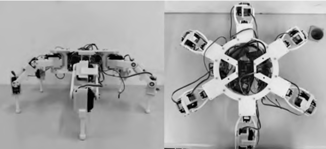
The robot prototype (Figure 3, conceptual description) features a graphite carbon body (weight: 5 kg) and ABS feet. Key specifications include:
- 18 servo motors (3 per leg, 30 N·m torque).
- IMU sensor for body orientation tracking.
- Foot-end pressure sensors with 0.1 N resolution .
Experiments were conducted on a flat surface, comparing the composite cycloid and Bézier curve trajectories over four cycles. Parameters included a 500 mm step length, 500 mm lift height, and 1-second phase duration .
7.2. Results and Analysis
Figures 4-7 (conceptual descriptions) present comparative data for pitch angle, roll angle, and angular velocities:
- Pitch Angle: Bézier curve showed ±2° variation vs. ±3° for cycloid, with reduced 抖动 .
- Roll Angle: Bézier curve limited variations to ±1.5°, compared to ±2.5° for cycloid, indicating better lateral stability .
- Angular Velocity: Bézier curve exhibited smoother transitions (±5°/s) versus abrupt spikes in the cycloid method (up to ±15°/s) .
Table 5. Quantitative stability comparison.
| Metric | Bézier Curve | Composite Cycloid | Improvement |
|---|---|---|---|
| Pitch angle range | ±2° | ±3° | 33% |
| Roll angle range | ±1.5° | ±2.5° | 40% |
| Max angular velocity | ±5°/s | ±15°/s | 67% |
These results confirm that the Bézier curve trajectory significantly enhances motion stability, aligning with the goals of advanced robot technology .
8. Conclusion
This study demonstrates the effectiveness of biomimetic design and Bézier curve trajectory optimization in improving hexapod robot stability. By replicating spider leg mechanics and adopting smooth foot trajectories, we achieved reduced impact forces and enhanced locomotion efficiency. The proposed approach offers a robust framework for robot technology, particularly in applications requiring reliable movement on uneven terrains.