
The design of conjugate tooth profiles is fundamental to the performance of the harmonic drive gear, a unique gearing system known for its compactness, high reduction ratios, and positional accuracy. Traditional design methods for the rigid wheel often rely on iterative calculations and post-manufacturing adjustments, which can be inefficient and may not yield optimal meshing characteristics. This article presents a comprehensive methodology for the design of rigid wheel tooth profiles based on an envelope simulation approach. By simulating the precise kinematic motion of the flexible wheel (flexspline) under the action of the wave generator, the conjugate profile of the stationary rigid wheel (circular spline) can be directly and efficiently derived. This method enhances design flexibility, allows for rapid analysis of key design parameters, and facilitates seamless integration with Computer-Aided Design (CAD) systems.
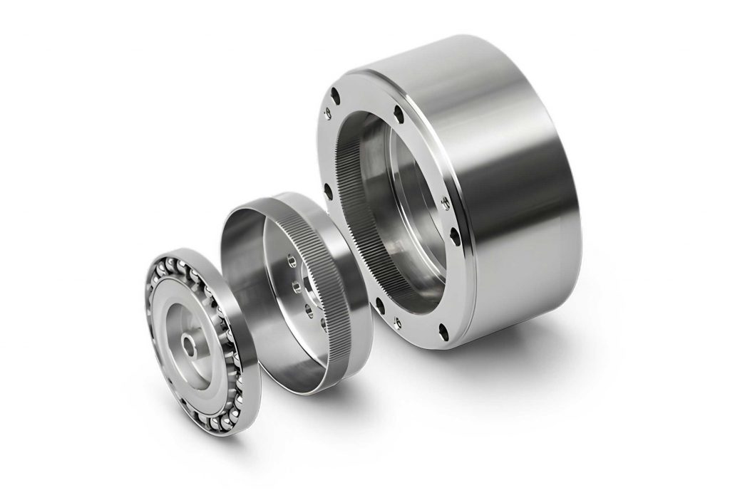
At the core of the harmonic drive gear operation is the elastic deformation of the flexible wheel. The wave generator, typically an elliptical bearing assembly, deforms the flexible wheel, causing its external teeth to engage with the internal teeth of the rigid wheel at two diametrically opposite regions. The kinematic relationship between these components is governed by well-established conjugate theory. For the purpose of rigid wheel profile generation, the flexible wheel tooth can be conceptualized as a cutting tool. As the flexible wheel undergoes its compound motion—a combination of radial deflection and tangential rotation—the envelope of all positions occupied by this “tool” defines the required conjugate profile of the rigid wheel.
Fundamentals of Conjugate Theory for Harmonic Drive Gears
To formulate the envelope simulation, we must first establish the coordinate systems and transformation laws. The flexible wheel profile is initially designed in its own coordinate system \((X_R, Y_R)\), often based on its neutral curve. The rigid wheel profile is derived in a fixed global coordinate system \((X_G, Y_G)\) centered at the wave generator’s rotation axis. The transformation from the flexible wheel coordinates to the rigid wheel coordinates involves both rotation and translation, dictated by the wave generator’s geometry and the pure-rolling condition between the flexible and rigid wheels.
The radial position \(\rho\) of a point on the flexible wheel’s neutral curve, relative to the wave generator center, is a function of the wave generator’s rotation angle \(\varphi_1\) and its elliptical geometry. If \(a\) and \(b\) are the semi-major and semi-minor axes of the wave generator, the radial displacement is given by:
$$\rho(\varphi_1) = \frac{ab}{\sqrt{b^2 + (a^2 – b^2) \sin^2(\varphi_1)}}$$
According to the no-slip condition, the arc length traveled by a point on the flexible wheel’s neutral curve must equal the arc length traveled on the rigid wheel’s pitch curve. This leads to the following integral relationship defining the rotation of the rigid wheel \(\varphi_2\):
$$\int_{0}^{\varphi_1} \sqrt{(\rho’)^2 + \rho^2} \, d\varphi = r_G \varphi_2$$
where \(r_G\) is the nominal radius of the rigid wheel’s pitch circle, and \(\rho’ = d\rho/d\varphi\). The difference angle \(\gamma\), which is crucial for the coordinate transformation, is defined as:
$$\gamma = \varphi_1 – \varphi_2 = \varphi_1 – \frac{1}{r_G} \int_{0}^{\varphi_1} \sqrt{(\rho’)^2 + \rho^2} \, d\varphi$$
The overall angular position \(\phi\) of the flexible wheel coordinate system relative to the rigid wheel system is then:
$$\phi = \arctan\left(\frac{\rho’}{\rho}\right) + \gamma$$
Finally, the family of curves representing the flexible wheel tooth profile positions in the rigid wheel coordinate system is given by the transformation matrix \(M\):
$$
\begin{bmatrix}
X_G(\theta, \varphi_1) \\
Y_G(\theta, \varphi_1) \\
1
\end{bmatrix} = M \cdot
\begin{bmatrix}
X_R(\theta) \\
Y_R(\theta) \\
1
\end{bmatrix} =
\begin{bmatrix}
\cos\phi & \sin\phi & \rho \sin\gamma \\
-\sin\phi & \cos\phi & \rho \cos\gamma \\
0 & 0 & 1
\end{bmatrix}
\begin{bmatrix}
X_R(\theta) \\
Y_R(\theta) \\
1
\end{bmatrix}
$$
where \(\theta\) is the parameter defining a point on the flexible wheel tooth profile. The envelope of this family of curves, satisfying the condition $$\frac{\partial X_G}{\partial \varphi_1} \frac{\partial Y_G}{\partial \theta} – \frac{\partial Y_G}{\partial \varphi_1} \frac{\partial X_G}{\partial \theta} = 0$$, yields the conjugate rigid wheel tooth profile.
Envelope Simulation Methodology and Implementation
The envelope condition, while analytically precise, can be computationally intensive to solve directly for complex flexible wheel profiles such as double-arc or S-shaped teeth. The simulation-based envelope method offers a robust and practical alternative. This method discretizes the motion of the harmonic drive gear and graphically constructs the envelope.
The simulation algorithm, implemented in a computational environment like MATLAB, follows these key steps:
- Profile Definition: Define the coordinates of the flexible wheel tooth profile \((X_R(\theta), Y_R(\theta))\). This profile can be an involute, double-arc, or any custom shape.
- Motion Discretization: Discretize the rotation of the wave generator into small angular increments \(\Delta \alpha\). For each wave generator position \(\alpha_i\), calculate the corresponding rigid wheel rotation \(\beta_i\) based on the transmission ratio (\(i = \alpha_i / \beta_i\)).
- Compound Motion Simulation: For each wave generator position, apply the compound motion to every point on the flexible wheel tooth profile. This involves two components:
- Tangential Motion: A rotation of the entire profile by angle \(\beta_i\) around the instantaneous center, approximated by \(\Delta x \approx (\beta_i \pi \rho_i) / 180\).
- Radial Motion: A displacement along the radial direction equal to the change in the wave generator’s radius vector: \(\Delta y = a – \rho(\alpha_i)\).
- Envelope Plotting: Plot the transformed position of the flexible wheel tooth profile for all wave generator positions \(\alpha_i\). The innermost boundary of this dense cluster of curves represents the envelope—the sought-after rigid wheel conjugate tooth profile.
The following table summarizes a typical set of input parameters for simulating a standard harmonic drive gear.
| Parameter | Symbol | Example Value | Unit |
|---|---|---|---|
| Module | \(m\) | 0.2 | mm |
| Number of Teeth (Flexible Wheel) | \(Z_F\) | 200 | – |
| Number of Teeth (Rigid Wheel) | \(Z_R\) | 202 | – |
| Transmission Ratio | \(i\) | 100 | – |
| Wave Generator Major Axis | \(a\) | Dependent on \(\omega^*\) | mm |
| Wave Generator Minor Axis | \(b\) | Dependent on \(\omega^*\) | mm |
| Radial Deformation Coefficient | \(\omega^*\) | Variable (0.8, 1.0, 1.2) | – |
Critical Analysis of Radial Deformation Coefficient (\(\omega^*\))
The radial deformation coefficient \(\omega^*\) is a paramount design parameter in any harmonic drive gear system. It is defined as the ratio of the maximum radial deformation of the flexible wheel \(\omega\) to the gear module \(m\):
$$\omega^* = \frac{\omega}{m}$$
where \(\omega = a – r_F\), and \(r_F\) is the nominal radius of the flexible wheel before deformation. The value of \(\omega^*\) directly determines the shape of the wave generator and profoundly influences the meshing performance. Envelope simulation provides an excellent tool for visualizing and quantifying these effects. The analysis below compares the meshing characteristics for three key values: \(\omega^* = 0.8, 1.0,\) and \(1.2\).
| Radial Coefficient (\(\omega^*\)) | Meshing Depth | Effective Mesh Zone | Risk of Tooth Jumping | Risk of Interference | Conjugate Profile Shape |
|---|---|---|---|---|---|
| 0.8 (Undercritical) | Shallower | Largest (more simultaneous tooth pairs) | Low | High (reduced tip clearance) | Broader, more relaxed curvature |
| 1.0 (Standard) | Moderate | Balanced | Moderate | Moderate | Standard conjugate shape |
| 1.2 (Overcritical) | Deepest | Reduced | High (increased tip clearance) | Low | Sharper, more pronounced curvature |
Interpretation of Results:
- Standard Design (\(\omega^* = 1.0\)): This represents a balanced design. The envelope simulation shows a well-defined conjugate profile with a sufficient number of curves forming the envelope, indicating a stable and predictable meshing zone. The tip clearance is adequate to avoid interference during the meshing-out phase.
- High Radial Coefficient (\(\omega^* = 1.2\)): Increasing \(\omega^*\) deepens the meshing engagement, which theoretically increases load-carrying capacity. However, the envelope simulation reveals a critical drawback: the number of curves contributing to the final envelope decreases significantly. This indicates a narrower effective meshing zone. Furthermore, the distance between the flexible wheel tooth tip and the generated rigid wheel tooth tip becomes excessively large during the meshing-out process, creating a high risk of tooth jumping or loss of contact, which is detrimental to motion transmission accuracy.
- Low Radial Coefficient (\(\omega^* = 0.8\)): Reducing \(\omega^*\) makes the wave generator more circular, which increases the number of teeth in simultaneous contact, potentially improving load distribution and compensating for transmission error. The simulation confirms a larger envelope zone. The trade-off, however, is a reduced meshing depth and, crucially, a very small tip clearance. This minimal clearance dramatically increases the risk of tip interference or scuffing between the tooth flanks of the harmonic drive gear components during operation.
The simulation conclusively demonstrates that the optimal design window for the radial deformation coefficient in a harmonic drive gear lies approximately between 0.8 and 1.2. Straying outside this window compromises performance by introducing significant risks of either jumping or interference.
Profile Extraction, Curve Fitting, and 3D Modeling
Once the envelope simulation is complete, the raw graphical output consists of a dense cluster of lines. The next step is to digitally extract the precise coordinates of the conjugate profile and convert them into a continuous curve suitable for CAD modeling.
1. Data Point Extraction: The envelope is defined as the inner boundary of the curve cluster. An algorithm is used to discretize the horizontal axis (\(X_G\)) and, for each \(x\)-coordinate, find the maximum \(Y_G\) value among all intersecting curves from the simulation. This set of \((X_{G_i}, Y_{G_i})\) points represents the discrete coordinates of the rigid wheel tooth flank.
$$P_{rigid} = \{ (X_{G_i}, Y_{G_i}) \ | \ Y_{G_i} = \max(Y_G(X_{G_i})) \text{ for all simulation curves} \}$$
2. Curve Fitting and Reconstruction: The discrete points \(P_{rigid}\) must be fitted with a smooth curve. Simple polynomial fitting (\(y = p_1x^n + … + p_{n+1}\)) can cause undesirable oscillations. A more stable approach is a weighted least-squares fit or a spline interpolation that minimizes the perpendicular distance variance from the data points, resulting in a smooth, accurate profile. The choice of fitting method can influence the final manufacturability and meshing smoothness of the harmonic drive gear.
| Fitting Method | Principle | Advantage for Harmonic Drive Gear Profile | Potential Drawback |
|---|---|---|---|
| Polynomial Fit | Minimizes vertical offset squared error. | Simple, generates a single analytic equation. | Can produce unrealistic waviness (Runge’s phenomenon) at the ends of the profile. |
| Weighted Least-Squares Spline | Minimizes weighted perpendicular distance error. | Produces a very smooth curve that follows the global data trend closely; ideal for CNC toolpath generation. | Does not guarantee interpolation of every data point. |
| Cubic Spline Interpolation | Passes through every data point with C² continuity. | Guarantees the profile passes through the simulated envelope points exactly. | Can be sensitive to noise in the extracted data points. |
3. CAD Model Generation: The fitted curve equation or coordinate set is exported to a CAD platform (e.g., Creo Parametric, SolidWorks). A single tooth profile is sketched using the imported geometry. This profile is then revolved around the gear axis and patterned circularly using the rigid wheel’s tooth count \(Z_R\) to create the complete internal tooth geometry. Subsequent Boolean operations with cylindrical solids yield the final 3D model of the rigid wheel component of the harmonic drive gear. This model is readily available for virtual assembly, tolerance analysis, Finite Element Analysis (FEA) for stress evaluation, and ultimately, for generating manufacturing instructions.
Conclusion and Advantages of the Envelope Simulation Method
The envelope simulation method for designing rigid wheel tooth profiles presents a significant advancement over traditional, formula-based approaches for harmonic drive gears. Its primary strength lies in its direct visualization of the meshing process and its high degree of flexibility. Key advantages include:
- Profile Agnosticism: The method is independent of the flexible wheel’s initial tooth form. Whether it’s an involute, double-arc, tri-arc, or any novel asymmetric profile, the conjugate rigid wheel profile is derived directly from its kinematic motion, ensuring perfect theoretical conjugation.
- Integrated Parameter Analysis: The impact of critical design parameters, most notably the radial deformation coefficient \(\omega^*\), can be instantaneously visualized and analyzed. Designers can rapidly iterate and optimize the design for specific goals such as maximizing contact ratio, ensuring safe tip clearance, or minimizing stress concentration.
- Seamless CAD/CAE Integration: The digital workflow from mathematical simulation to fitted curve to 3D CAD model is straightforward. This digital thread enables rapid prototyping, advanced stress and thermal simulations, and precision manufacturing, significantly shortening the development cycle for custom or high-performance harmonic drive gear systems.
- Enhanced Understanding: The graphical output of the simulation provides an intuitive understanding of the meshing zone, the path of contact, and potential problem areas like undercutting or inadequate clearance, which might be less obvious in purely numerical solutions.
In summary, the adoption of envelope simulation represents a more efficient, accurate, and versatile paradigm for the design and analysis of harmonic drive gear transmissions. By leveraging computational power to simulate the fundamental kinematics of conjugation, it allows engineers to push the boundaries of performance, reliability, and miniaturization in applications ranging from robotic actuators to aerospace mechanisms.