
In modern engineering applications, such as aerospace, industrial robotics, and precision instrumentation, the harmonic drive gear stands out due to its compact size, high transmission ratio, and substantial load capacity. However, in practical operations, factors like wear and deformation often lead to reduced transmission accuracy and poor reliability, directly impacting the overall lifespan and performance of equipment. This paper aims to address these challenges by establishing a comprehensive transmission error model that incorporates both static and dynamic influences, including wear and deformation. Through reliability analysis and optimization design, we seek to enhance the precision and durability of harmonic drive gears under realistic working conditions.
The harmonic drive gear primarily consists of three key components: the circular spline (rigid gear), the flexspline (flexible gear), and the wave generator. The wave generator, typically an elliptical cam, deforms the flexspline, causing it to mesh with the circular spline at specific points, thereby enabling motion transmission with high reduction ratios. Despite its advantages, the transmission accuracy is compromised by various errors, which can be categorized into static errors (from manufacturing and assembly) and dynamic errors (from wear and deformation during operation).
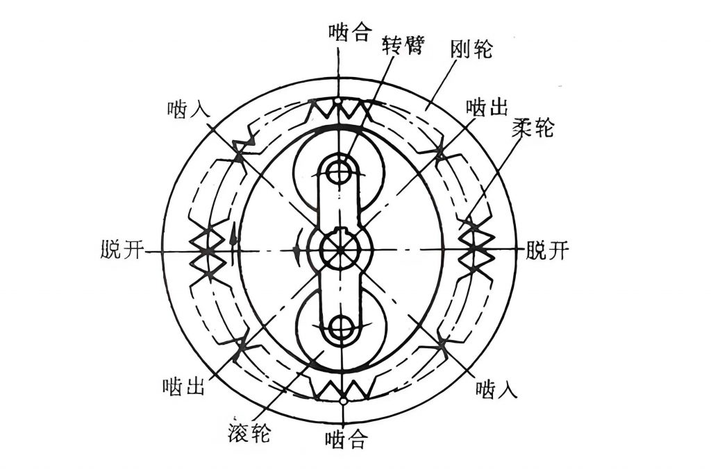
To systematically analyze these effects, we first develop a transmission error model. The total transmission error angle, denoted as \(\Delta \theta_{out}\), is derived from the cumulative impact of individual error sources. The static errors include manufacturing inaccuracies such as pitch deviation and tangential composite error for both the circular spline and flexspline, as well as assembly errors like radial runout and fit clearance. The dynamic errors arise from wear at the interface between the flexspline inner wall and the flexible bearing outer race, and from the periodic deformation of the flexspline due to the wave generator’s action.
The general expression for the transmission error angle is given by:
$$
\Delta \theta_{out} = \frac{k_b}{\sqrt{N}} \times \frac{206.4}{d_1} \times \frac{\sqrt{\Delta F_{p1}^2 + \Delta F_{p2}^2 + \Delta f_{f1}^2 + \Delta f_{f2}^2 + \sum e_i^2 + (e_{WG1} + V(T, v, t))^2 + (e_{WG2} + B(T, v))^2}}{\cos^2 \alpha_n}
$$
where:
- \(\Delta F_{p1}, \Delta F_{p2}\) are the cumulative pitch errors of the circular spline and flexspline, respectively.
- \(\Delta f_{f1}, \Delta f_{f2}\) are the tangential composite errors of the circular spline and flexspline.
- \(e_i\) represents other static errors from fit clearances and radial runouts.
- \(e_{WG1}\) and \(e_{WG2}\) are errors associated with the wave generator, including radial clearance and runout.
- \(V(T, v, t)\) is the dynamic wear volume, a function of output load \(T\), input speed \(v\), and operating time \(t\).
- \(B(T, v)\) is the maximum radial displacement due to flexspline deformation, dependent on load and speed.
- \(k_b\) is a correlation coefficient, \(N\) is the number of simultaneously meshing tooth pairs, \(d_1\) is the pitch diameter of the driven gear, and \(\alpha_n\) is the pressure angle.
This model integrates both static imperfections and time-varying dynamic factors, providing a foundation for accuracy reliability assessment.
Wear is a critical dynamic factor that progressively degrades the performance of the harmonic drive gear. The primary wear occurs at the contact between the flexspline inner wall and the flexible bearing outer race, where mixed lubrication conditions prevail, leading to adhesive and abrasive wear mechanisms. An empirical wear model based on the Archard formulation is often used, but it fails to account for the impact of cyclic loading and flexible deformation inherent in harmonic drive gear operation. To improve accuracy, we employ a Bayesian calibration approach to refine the empirical model using experimental wear data.
The Bayesian-corrected wear model is expressed as:
$$
V_{re}(T’, v’, t’) = V_{or}(T’, v’, t’) + \Delta V^*(T’, v’, t’) + \epsilon_V
$$
where \(V_{or}\) is the original empirical wear model, \(\Delta V^*\) is the wear deviation predicted via Gaussian Process (GP) regression, and \(\epsilon_V\) is a random error term following a normal distribution. The GP model is trained on experimental data correlating wear volume with operational parameters (load, speed, time). The wear rate \(\phi\) in the empirical model is given by:
$$
\phi = \frac{dV}{dt} = \frac{2 k_e k_s W f}{3 \sigma_s (f_B – f_E)} \left(1 + 3(f – f_E)^2\right)^{1/2}
$$
where \(k_e, k_s\) are constants, \(W\) is the load per asperity, \(\sigma_s\) is the yield stress, and \(f_B, f_E, f\) are friction coefficients under boundary, full-film, and mixed lubrication, respectively.
Experimental wear tests were conducted on a specific harmonic drive gear under varying loads and speeds. The measured wear volumes after different operating durations are summarized in the table below, showcasing the nonlinear progression of wear.
| Test ID | Output Load \(T\) (N·m) | Input Speed \(v\) (r/min) | Operating Time \(t\) (h) | Wear Volume \(V\) (μm) |
|---|---|---|---|---|
| 1 | 17.5 | 300 | 550 | 2.98 |
| 2 | 38.0 | 100 | 550 | 3.85 |
| 3 | 25.0 | 300 | 1200 | 5.34 |
| 4 | 17.5 | 100 | 1750 | 5.09 |
| 5 | 25.0 | 500 | 1750 | 7.12 |
| 6 | 38.0 | 300 | 2150 | 9.83 |
| 7 | 25.0 | 300 | 3250 | 10.02 |
| 8 | 38.0 | 500 | 3250 | 11.17 |
| 9 | 17.5 | 300 | 3650 | 9.79 |
The GP regression model for wear deviation \(\Delta V^*\) is constructed as a Gaussian process:
$$
\Delta V^* = \mathbf{y}'(T’, v’, t’) \mid T, v, t, \mathbf{y} \sim \mathcal{N}\left( \mathbf{K}_*^T (\mathbf{K} + \sigma^2 \mathbf{E})^{-1} \mathbf{y}, \mathbf{K}_{**} – \mathbf{K}_*^T (\mathbf{K} + \sigma^2 \mathbf{E})^{-1} \mathbf{K}_* \right)
$$
where \(\mathbf{K}\) is the covariance matrix of training inputs, \(\mathbf{K}_*\) is the covariance between training and prediction inputs, and \(\mathbf{y}\) is the vector of training outputs (wear deviations). This approach allows accurate prediction of wear under untested conditions, validated by ensuring that experimental data points lie within the 95% confidence interval of predictions.
Another significant dynamic factor is the deformation of the flexspline. During operation, the flexspline undergoes cyclic elastic deformation due to the wave generator’s elliptical motion, contributing to high-frequency components of transmission error. To quantify this, we conducted transmission tests measuring the maximum radial displacement \(B\) at the flexspline cup mouth under various loads and speeds. A GP regression model is similarly employed to predict \(B\) as a function of load and speed, since analytical formulas are complex and data is limited.
The flexspline deformation prediction model is:
$$
B_{pre} = B'(T’, v’) \mid T, v, B \sim \mathcal{N}\left( \mathbf{K}_{B*}^T (\mathbf{K}_B + \sigma_B^2 \mathbf{E})^{-1} B, \mathbf{K}_{B**} – \mathbf{K}_{B*}^T (\mathbf{K}_B + \sigma_B^2 \mathbf{E})^{-1} \mathbf{K}_{B*} \right)
$$
where the covariance matrices are defined analogously to the wear model. Experimental validation confirms that predicted radial displacements align well with measured values, enabling reliable integration into the overall error model.
With the transmission error model, dynamic wear model, and flexspline deformation model established, we proceed to accuracy reliability analysis. The performance function for reliability is defined as:
$$
g(\mathbf{a}, \theta_{al}) = \Delta \theta_{out} – \theta_{al}
$$
where \(\mathbf{a} = (T, v, t)\) represents operational parameters, and \(\theta_{al}\) is the allowable transmission error. Failure occurs when \(g > 0\), and the reliability \(P\) is the probability that \(g \leq 0\). Given the complexity and high dimensionality of the model, direct Monte Carlo simulation (MCS) would be computationally expensive. Therefore, we employ a surrogate modeling approach using Kriging (Gaussian process regression) combined with Latin Hypercube Sampling (LHS) to efficiently approximate the response surface.
The LHS method partitions each input variable range into intervals, ensuring stratified sampling. A set of training samples \(\mathbf{K}'(\mathbf{a}, \Delta \theta)\) is generated, and a Kriging model is trained to predict the transmission error for any input \(\mathbf{w} = (T_x, v_x, t_x)\):
$$
J(\mathbf{w}) = \text{Kriging}(\mathbf{w}, \mathbf{K}'(\mathbf{a}, \Delta \theta))
$$
Then, MCS with \(N\) samples is performed on the Kriging surrogate to estimate reliability:
$$
P = 1 – P_f = 1 – \frac{n(g(J(\mathbf{w}), \theta_{al}) > 0)}{N}
$$
where \(n\) is the count of failed samples. For a case study with operational parameters \(T = 17.5 \, \text{N·m}\), \(v = 100 \, \text{r/min}\), and an allowable error \(\theta_{al} = 1 \, \text{arc-min}\), the reliability over time is computed. The results show that reliability decreases gradually initially but drops significantly after prolonged operation, reaching approximately 91.17% at \(t = 3000 \, \text{h}\), indicating a need for design optimization.
To enhance the harmonic drive gear’s reliability, we formulate a reliability-based optimization design problem. The goal is to minimize manufacturing cost while ensuring that reliability meets a specified threshold and wear volume remains within limits. First, sensitivity analysis is performed on the error parameters to identify the most influential ones, reducing the number of design variables. The relative sensitivity \(\Delta s_i\) of each error parameter to transmission error is computed as:
$$
s_i = \frac{\partial \Delta \theta}{\partial \Delta e_i}, \quad \Delta s_i = \frac{s_i}{\sum_{i=1}^{12} s_i}
$$
The analysis reveals that parameters such as cumulative pitch errors (\(\Delta F_{p1}, \Delta F_{p2}\)) and certain fit clearances (\(e_{CS12}\)) have high sensitivity, while others like tangential composite errors (\(\Delta f_{f1}, \Delta f_{f2}\)) have lower impact. Based on this, eight key error parameters are selected as design variables.
The optimization problem is mathematically stated as:
$$
\begin{aligned}
& \underset{\Delta \mathbf{e}’}{\text{minimize}} & & C(\Delta \mathbf{e}’) = \sum_{i=1}^{8} k_j C_j(e’_i) \\
& \text{subject to} & & P(\Delta \mathbf{e}’)(T, v, t) \geq P_{re} \\
& & & V(\Delta \mathbf{e}’, (T, v, t)) = V_{ac} – V_{pre} \leq 0 \\
& & & \delta_{min} \leq e’_i \leq \delta_{max}
\end{aligned}
$$
where:
- \(C(\Delta \mathbf{e}’)\) is the total manufacturing cost, composed of cost functions for dimensional tolerance \(C_1\), geometric tolerance \(C_2\), and runout tolerance \(C_3\).
- \(P_{re}\) is the required reliability (e.g., 99% at 3000 hours).
- \(V_{pre}\) is the permissible wear volume.
- \(\delta_{min}, \delta_{max}\) define the allowable tolerance ranges for each design variable.
The cost functions are empirically derived:
$$
C_1(\Delta e’_i) = a_{e’_i} – b_{e’_i} Z_{e’_i} + \frac{e_{e’_i}}{c_{e’_i} \times Z_{e’_i} + d_{e’_i}}, \quad C_2(\Delta e’_i) = f_{e’_i} e^{-g_{e’_i} Z_{e’_i}} + \frac{h_{e’_i}}{Z_{e’_i}^{l_{e’_i}}}, \quad C_3(\Delta e’_i) = m_{e’_i} e^{-s_{e’_i} Z_{e’_i}}
$$
where \(Z_{e’_i}\) is the tolerance value, and other symbols are cost coefficients specific to manufacturing processes.
We apply the Sequential Quadratic Programming (SQP) algorithm to solve this nonlinear constrained optimization problem. For the case study, the initial and optimized tolerance values for the design variables are compared in the table below.
| Error Parameter | Initial Tolerance (μm) | Optimized Tolerance (μm) |
|---|---|---|
| \(\Delta F_{p1}\) (circular spline pitch error) | 36 | 32.4 |
| \(\Delta F_{p2}\) (flexspline pitch error) | 36 | 31.3 |
| \(e_{CS12}\) (fit clearance) | 45 | 38.7 |
| \(\Delta f_{f1}\) (circular spline tangential error) | 16 | 16.7 |
| \(\Delta f_{f2}\) (flexspline tangential error) | 16 | 16.7 |
| \(e_{CS11}\) (radial runout) | 12 | 13.3 |
| \(e_{FS12}\) (output shaft runout) | 12 | 13.2 |
| \(e_{WG21}\) (wave generator clearance) | 15 | 15.4 |
The optimization results show that the total manufacturing cost increases slightly from 319.22 units to 324.65 units, a marginal rise of 1.70%. However, the reliability at \(t = 3000 \, \text{h}\) under the specified operational conditions improves significantly from 91.17% to 99.02%, an enhancement of 7.85 percentage points. This demonstrates that by intelligently allocating tolerances—tightening critical parameters while loosening less sensitive ones—the harmonic drive gear can achieve high reliability without substantial cost escalation.
In conclusion, this study presents a holistic framework for analyzing and optimizing the accuracy reliability of harmonic drive gears, incorporating both wear and deformation dynamics. The integrated model, combining static errors, Bayesian-corrected wear prediction, and GP-based deformation estimation, provides a realistic representation of transmission error evolution. The reliability analysis via Kriging surrogate and MCS efficiently quantifies performance degradation over time. The optimization design, guided by sensitivity analysis and cost-reliability trade-offs, yields a practical solution for enhancing harmonic drive gear durability. Future work could explore additional dynamic factors like lubrication degradation or temperature effects, and extend the methodology to other precision gear systems. The approach underscores the importance of considering time-varying factors in the design of high-reliability mechanical transmissions, ensuring that harmonic drive gears continue to meet the stringent demands of advanced engineering applications.