
Harmonic drive gears are a critical component in precision motion control systems, notably within solar array drive assemblies (SADA) for spacecraft. Their advantages, including high reduction ratios in compact stages, near-zero backlash, high torque capacity, and excellent positional accuracy, make them indispensable for space applications where mass, volume, and reliability are paramount. However, the operational life of these components in such critical applications is challenged by various degradation mechanisms. Factors such as wear in the tooth meshing zones, fatigue under cyclic loading, and the impact of the space environment (e.g., vacuum, thermal cycling) can lead to a gradual decline in the structural strength of key components, primarily the flexspline. Traditional optimal design methods often treat material strength as a static, time-invariant property. This assumption can lead to non-conservative designs that may not meet reliability targets over the intended mission life. Therefore, performing a reliability-based design optimization (RBDO) that explicitly accounts for the time-dependent degradation of strength is essential for developing more robust and safer harmonic drive gear systems.
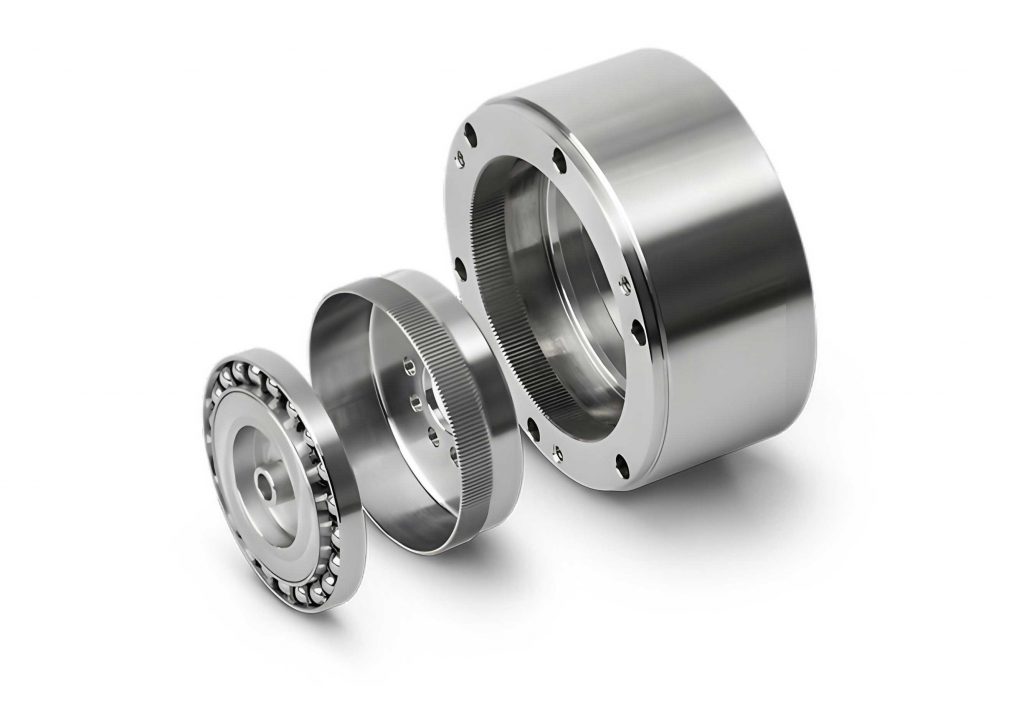
The core of a harmonic drive gear system consists of three elements: the circular spline (rigid outer ring), the flexspline (thin-walled, flexible cup with external teeth), and the wave generator (elliptical bearing assembly). During operation, the wave generator deforms the flexspline into an elliptical shape, causing its external teeth to engage with the internal teeth of the circular spline at two diametrically opposite regions. The difference in the number of teeth between the flexspline and circular spline creates the high reduction ratio. This working principle subjects the flexspline to continuous cyclic elastic deformation, making its fatigue strength the primary limiting factor for the life of the entire harmonic drive gear assembly.
Strength degradation in mechanical components like the flexspline is a stochastic process characterized by monotonicity and randomness. Monotonicity implies that the material’s resistance to stress only decreases over time due to cumulative damage and cannot recover. Randomness signifies that the exact path of degradation for any individual component is unpredictable, influenced by inherent material inhomogeneities and variable operational loads. Common stochastic processes like Brownian motion or the Wiener process allow for negative increments and are thus unsuitable for modeling pure degradation. For modeling gradual, monotonic deterioration, the Gamma process has been established as a mathematically appropriate and empirically validated tool. A Gamma process \(\{D(t), t \geq 0\}\) is a stochastic process with independent, non-negative increments, where the increment over a time interval \((s, t]\) follows a Gamma distribution.
Let \(X\) be a random variable following a Gamma distribution. Its probability density function is given by:
$$f_X(x; \alpha, \beta) = \frac{\beta^{\alpha}}{\Gamma(\alpha)} x^{\alpha-1} e^{-\beta x} I_{(0, \infty)}(x)$$
where \(\alpha > 0\) is the shape parameter, \(\beta > 0\) is the scale parameter, \(\Gamma(\cdot)\) is the Gamma function, and \(I_A(x)\) is the indicator function. A Gamma process \(D(t)\) has the following properties: \(D(0) = 0\); it has independent increments; and for \(t > s \geq 0\), the increment \(D(t) – D(s) \sim \Gamma(\alpha(t) – \alpha(s), \beta)\). The mean and variance of the degradation at time \(t\) are \(\mathbb{E}[D(t)] = \alpha(t)/\beta\) and \(\text{Var}[D(t)] = \alpha(t)/\beta^2\), respectively. The shape function \(\alpha(t)\) is often chosen as a power law, \(\alpha(t) = c t^b\), or a linear function, \(\alpha(t) = a t\), for simplicity. In the context of the harmonic drive gear flexspline, we model the fatigue strength \(S\) as an initial strength \(S_0\) minus a Gamma degradation process: \(S(t) = S_0 – D(t)\). The time-dependent reliability \(R(t)\), defined as the probability that the strength remains greater than the applied stress \(\sigma\), is then:
$$R(t) = \Pr(S(t) > \sigma) = \Pr(S_0 – D(t) > \sigma) = F_{D(t)}(S_0 – \sigma)$$
where \(F_{D(t)}(\cdot)\) is the cumulative distribution function of the Gamma degradation at time \(t\).
The objective of the optimal design is to minimize the volume (and thus mass) of the harmonic drive gear‘s flexspline, a crucial goal for aerospace applications, while ensuring all reliability and functional constraints are satisfied throughout its service life. The primary design variables are the key geometric parameters of the flexspline:
$$\mathbf{d} = [m, l, \delta, b]^T = [d_1, d_2, d_3, d_4]^T$$
where \(m\) is the gear module, \(l\) is the cup length, \(\delta\) is the wall thickness of the flexspline, and \(b\) is the face width. The volume of the flexspline cup can be expressed as a function of these variables:
$$V(\mathbf{d}) = \pi b \left[d_r + d_3 + m(h_a^* + c^*)\right]\left[d_r + 2d_3 + m(h_a^* + c^*)\right] – 0.816\pi d_3 (l – b)\left[1.044z_1 – 2(h_a^* + c^*) – \frac{d_3}{m}\right]$$
where \(d_r\) is the inner radius of the flexspline cup, \(h_a^*\) is the addendum coefficient, \(c^*\) is the clearance coefficient, and \(z_1\) is the number of teeth on the flexspline.
The design is subject to a comprehensive set of 21 constraints \(c_i(\mathbf{d}, \mathbf{x}, \mathbf{y}) \geq 0.98\), encompassing static and dynamic reliability requirements, geometric compatibility, and manufacturing limits. Here, \(\mathbf{x}\) represents random variables (e.g., material fatigue limits \(\sigma_{-1}, \tau_{-1}\), load torque \(T_0\)), and \(\mathbf{y}\) represents interval or fuzzy variables (e.g., stress concentration factors \(K_\sigma, K_\tau\), load distribution factor \(K\)). The constraints ensure the harmonic drive gear operates safely and efficiently. A subset of the key reliability constraints is summarized in the table below.
| Constraint Category | Constraint Function (Simplified Form) | Description |
|---|---|---|
| Flexspline Fatigue (Shear & Bending) | $$\Pr\left(g_1(\mathbf{d},\mathbf{x},\mathbf{y}) = \frac{16}{\pi} \left( \frac{q_1}{m^4} + \frac{q_2}{\delta^2 m^2} + \frac{q_3}{l^2} \right)^{-1} – \tau_{-1} \geq 0 \right)$$ | Ensures combined shear stress from torsion and bending is below the time-varying fatigue strength with high probability. |
| Load Capacity (Surface Durability) | $$\Pr\left(g_2(\mathbf{d},\mathbf{x},\mathbf{y}) = \frac{1.5}{4\epsilon} b m z_1 p_p – T_0 \geq 0 \right)$$ | Prevents surface pitting by limiting contact pressure. |
| Buckling Stability | $$\Pr\left(g_5(\mathbf{d},\mathbf{x},\mathbf{y}) = \delta – \frac{T E l^2}{2.8 r_m^3} \left[ 2.6 + 1.4\left(\frac{l}{r_m}\right)^2 + \frac{2\pi^2 r_m^2}{(1-\nu^2)l^2} \right]^{-1/2} \geq 0 \right)$$ | Prevents elastic instability of the thin-walled cup under radial deformation. |
| Tooth Interference | $$\Pr(g_7 \geq 0), \Pr(g_8 \geq 0), \Pr(g_9 \geq 0)$$ | Series of geometric constraints preventing interference during meshing and assembly. |
| Geometric Limits | $$\Pr(0.3 \leq m \leq 1.0), \Pr(0.01m z_1 \leq \delta \leq 0.03m z_1), \Pr(0.8m z_1 \leq l \leq 1.1m z_1)$$ | Practical bounds on design variables from manufacturing and assembly. |
The traditional, or static, RBDO model does not incorporate strength degradation. It seeks to find the optimal design vector \(\mathbf{d}^*\) that minimizes volume subject to the constraints being satisfied at time \(t=0\) (or for a fixed strength value):
$$
\begin{aligned}
& \min_{\mathbf{d}, \mathbf{x}, \mathbf{y}} && V(\mathbf{d}) \\
& \text{s.t.} && c_i(\mathbf{d}, \mathbf{x}, \mathbf{y}) = \Pr(g_i(\mathbf{d}, \mathbf{x}, \mathbf{y}) \geq 0) \geq R_{\text{min}}, \quad i=1,2,…,21.
\end{aligned}
$$
To account for the inevitable wear and fatigue damage in the harmonic drive gear during its mission life, we formulate a dynamic RBDO model. The core modification is that the strength in the stress-strength interference model is now a function of time, \(S(t) = S_0 – D(t)\), where \(D(t)\) follows a Gamma process. The key reliability constraint (like the fatigue constraint \(g_1\)) becomes time-dependent. The optimization must ensure that the reliability at the end of the design life \(t_L\) (e.g., 5 years) meets the minimum requirement \(R_{\text{target}}\). This forces the initial design to have a higher intrinsic reliability \(R(0)\) to compensate for the degradation over time. The dynamic RBDO model is:
$$
\begin{aligned}
& \min_{\mathbf{d}, \mathbf{x}, \mathbf{y}} && V(\mathbf{d}) \\
& \text{s.t.} && c_1(\mathbf{d}, \mathbf{x}, \mathbf{y}, t_L) = \Pr(S_0 – D(t_L) > \sigma(\mathbf{d},\mathbf{x},\mathbf{y})) \geq R_{\text{target}} \\
& && c_i(\mathbf{d}, \mathbf{x}, \mathbf{y}) = \Pr(g_i(\mathbf{d}, \mathbf{x}, \mathbf{y}) \geq 0) \geq R_{\text{min}}, \quad i=2,3,…,21.
\end{aligned}
$$
For a numerical illustration, consider a design case where the Gamma process parameters for strength degradation are estimated from historical data or accelerated testing, resulting in a mean degradation rate. Suppose the requirement is that the reliability after 5 years of operation must be at least \(R(5)=0.92\). Using a linear shape function \(\alpha(t) = a t\) for the Gamma process, the reliability function \(R(t)\) can be computed. The table below shows a hypothetical decay of reliability from its initial value.
| Time, \(t\) (years) | Reliability, \(R(t)\) |
|---|---|
| 0 | 0.980 |
| 1 | 0.970 |
| 2 | 0.960 |
| 3 | 0.948 |
| 4 | 0.935 |
| 5 | 0.920 |
To meet \(R(5)=0.92\), the initial design must have \(R(0) \approx 0.98\). Solving both the static model (with \(R_{\text{min}}=0.92\)) and the dynamic model (with \(R_{\text{target}}=0.92\) at \(t_L=5\)) using numerical optimization techniques (e.g., MATLAB’s `fmincon` with reliability analysis loops using First Order Reliability Method – FORM) yields the following optimal design parameters:
| Design Variable | Static RBDO Result | Dynamic RBDO (with Degradation) Result |
|---|---|---|
| Module, \(m\) (mm) | 0.80 | 0.80 |
| Cup Length, \(l\) (mm) | 154.8 | 156.7 |
| Face Width, \(b\) (mm) | 27.1 | 27.1 |
| Wall Thickness, \(\delta\) (mm) | 1.94 | 1.96 |
| Flexspline Volume, \(V\) (mm³) | 2,689,168 | 2,698,269 |
The results clearly demonstrate that the dynamic RBDO model, which accounts for strength degradation, produces a more conservative design compared to the static model. While the module and face width remain unchanged, the dynamic model requires a slightly longer cup length and a thicker wall to build in a higher initial strength (and thus higher initial reliability \(R(0)=0.98\)) to ensure the reliability threshold is still met after 5 years of degradation. This results in a small increase of approximately 0.34% in the calculated volume. This conservatism is not a drawback but rather a reflection of a more realistic and safer design philosophy for critical, long-life components like the harmonic drive gear in a SADA. The static model, by ignoring degradation, risks producing an optimized design that may meet reliability goals only at the beginning of life but could fall below the required threshold before the end of the mission, posing a significant risk of failure.
In conclusion, the consideration of time-dependent strength degradation through stochastic processes like the Gamma process is crucial for the accurate reliability assessment and optimal design of long-life mechanical systems. For harmonic drive gears used in aerospace applications, a dynamic RBDO framework ensures that the design is not only optimal in terms of mass and size at the initial stage but also reliably satisfies all performance and safety constraints throughout its entire operational lifespan. This approach leads to more robust, reliable, and ultimately safer designs, as it explicitly plans for the inevitable material deterioration that occurs in service. The resulting designs may be marginally heavier or larger than those from a static analysis, but this is the necessary premium for guaranteeing long-term performance and avoiding in-service failures in missions where repair is often impossible.