
The strain wave gear drive, also known as the harmonic drive, represents a pivotal advancement in precision motion control technology. Its unique operating principle, based on the controlled elastic deformation of a flexible gear, enables exceptional performance characteristics. This article presents an in-depth analysis of the relationship between the deformation of the cup-type flexible gear and the force required to induce that deformation. We establish a theoretical model, validate it through meticulous experimentation, and employ MATLAB for sophisticated data analysis and model refinement. The ultimate goal is to provide a reliable theoretical foundation for the design of advanced components, such as novel elastic wave generators, which aim to optimize the meshing conditions within the strain wave gear assembly.
Fundamentals of Strain Wave Gear Operation
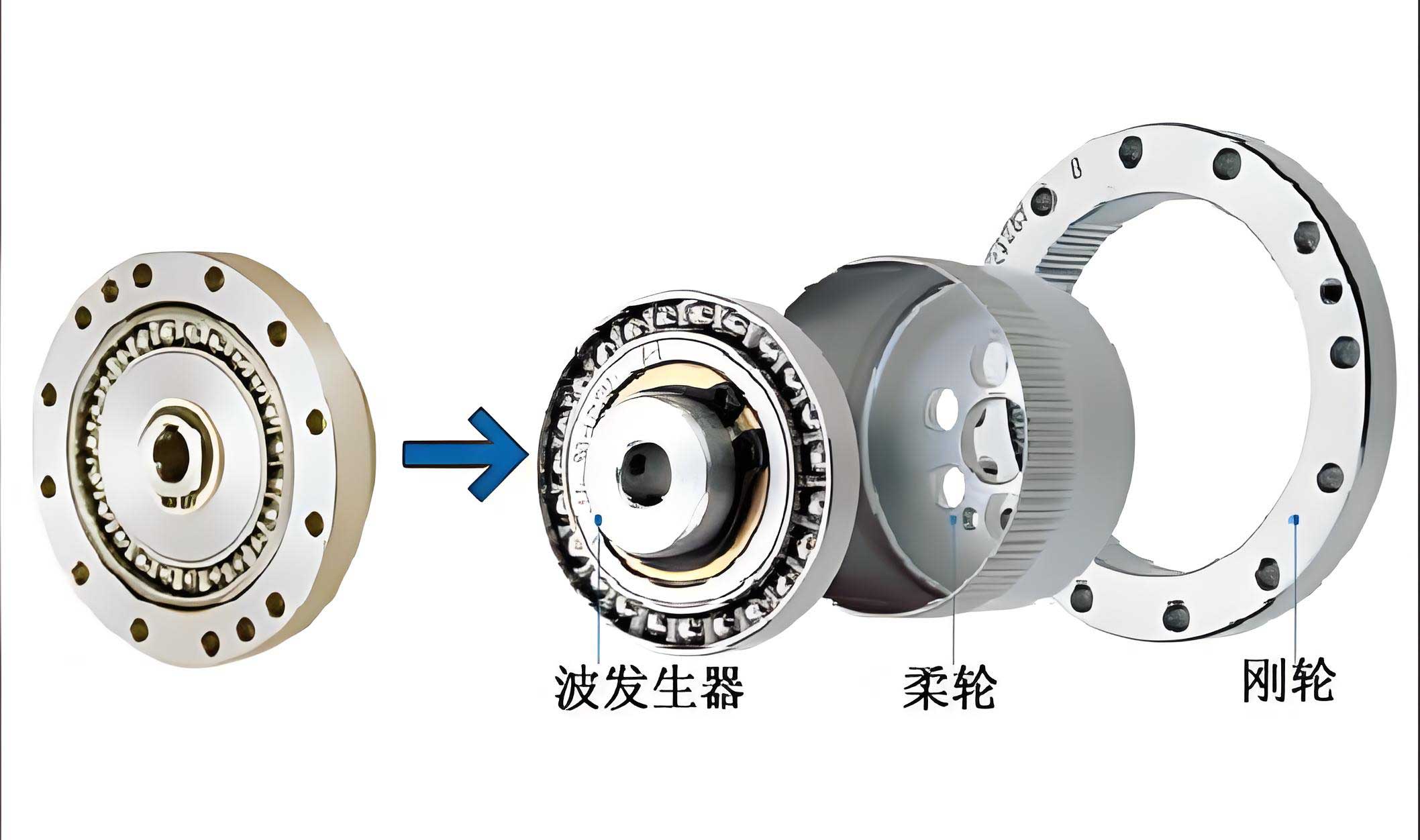
A standard strain wave gear transmission consists of three primary components: the wave generator, the flexible spline (or flexspline/cup), and the circular spline. The flexible spline is a thin-walled, externally toothed cup, while the circular spline is a rigid, internally toothed ring. Critically, the flexible spline has fewer teeth (typically by two) than the circular spline. Prior to assembly, the flexible spline has a perfect circular cross-section. The wave generator, which is elliptical in shape, is inserted into the bore of the flexible spline, forcing it to conform to its elliptical shape. This elastic deformation causes the teeth of the flexible spline to engage with those of the circular spline at two diametrically opposite regions, corresponding to the major axis of the ellipse.
The relative motion is achieved because the wave generator’s rotation causes the engagement zones to propagate around the circumference. For each full rotation of the wave generator, the flexible spline rotates backward relative to the circular spline by an amount equal to the difference in their number of teeth. This principle grants the strain wave gear its high reduction ratios, compact size, zero-backlash capability, and high torque capacity. The central element enabling this mechanism is the controlled, non-linear elastic deformation of the flexible spline, making its mechanical behavior the cornerstone of transmission design and performance.
Mathematical Modeling of Flexible Gear Deformation
To quantitatively analyze the flexible gear’s behavior, we must establish a mathematical relationship between the radial deformation (ω) and the deforming force (P). The flexible gear is a complex component featuring a toothed rim connected to a cylindrical shell. A direct analytical solution considering the detailed tooth geometry is exceedingly complex. Therefore, a common and effective simplification in strain wave gear analysis is to model the flexible gear as an equivalent smooth, thin-walled cylindrical shell. This approach focuses on the deformation of the neutral axis of the shell, which is adequate for deriving the primary deformation-force relationship.
The analysis is based on the moment theory of cylindrical shells and rests on the following key assumptions:
- The elastic deformation state of the flexible gear’s neutral axis under the deforming and meshing forces is stable and invariant.
- The elastic deformations are considered small.
- During operation, the length of the neutral axis of the flexible gear remains constant (neither extends nor contracts).
We consider the geometry of the cylindrical shell model. Let \( u \), \( v \), and \( w \) represent the displacements in the axial (z), circumferential (φ), and radial directions, respectively. According to shell theory and the condition of zero mid-surface strain, we have the geometric equations:
$$
\begin{align*}
\epsilon_z &= \frac{\partial u}{\partial z} = 0 \\
\epsilon_\varphi &= \frac{1}{R} \left( \frac{\partial v}{\partial \varphi} + w \right) = 0 \\
\gamma &= \frac{\partial v}{\partial z} + \frac{1}{R} \frac{\partial u}{\partial \varphi} = 0
\end{align*}
$$
where \( \epsilon_z \), \( \epsilon_\varphi \), and \( \gamma \) are the axial strain, circumferential strain, and shear strain of the mid-surface, respectively, and \( R \) is the radius of the neutral axis of the cylindrical shell.
Employing the energy method from elasticity theory, we introduce the cylindrical stiffness \( D \):
$$ D = \frac{E \delta^3}{12(1-\nu^2)} $$
where \( E \) is Young’s modulus, \( \delta \) is the wall thickness of the shell, and \( \nu \) is Poisson’s ratio. The governing bending differential equation can be expressed as:
$$ \frac{d^2w}{d\varphi^2} + w = -\frac{M_\varphi R^2}{D(1-\nu^2)} $$
To solve this, the radial displacement \( w \) is expressed as a trigonometric series, representing the elliptical deformation mode and its harmonics:
$$ w = \sum_{n=1,2,3,\ldots}^{\infty} (a_n \sin n\varphi + b_n \cos n\varphi) $$
For a deformation symmetric about the major axis and dominated by the fundamental elliptical mode (n=2), and considering a radial force distribution, the solution for the radial displacement due to a concentrated deforming force per unit length can be derived. The resulting expression for the theoretical radial displacement is:
$$ w = \frac{2 P R^3}{\pi D (1-\nu^2)} \sum_{n=2,4,6,\ldots}^{\infty} \frac{\cos n\varphi}{(n^2-1)^2} $$
From this, the theoretical deforming force \( P \) required to produce a given nominal radial deformation \( \omega_0 \) (the difference between the major and minor radii) is obtained by integrating the work done. The resulting theoretical model for the deforming force is:
$$ P = \frac{\pi E \omega_0 \delta^3}{24 R^3} \sum_{n=2,4,6,\ldots}^{\infty} \frac{1}{(n^2-1)^2} $$
This model reveals crucial design insights for the strain wave gear: the initial deforming force \( P \) is directly proportional to the cube of the flexible gear’s wall thickness (\( \delta^3 \)) and its material’s Young’s modulus (\( E \)), and directly proportional to the radial deformation (\( \omega_0 \)). It is inversely proportional to the cube of its nominal radius (\( R^3 \)). The series summation converges quickly, with the n=2 term being dominant. Calculating this sum:
$$ S = \sum_{n=2,4,6,\ldots}^{\infty} \frac{1}{(n^2-1)^2} = \frac{1}{(2^2-1)^2} + \frac{1}{(4^2-1)^2} + \frac{1}{(6^2-1)^2} + \ldots \approx \frac{1}{9} + \frac{1}{225} + \frac{1}{1225} \approx 0.123 $$
Thus, the theoretical force equation simplifies approximately to:
$$ P_{theory} \approx 0.123 \times \frac{\pi E \omega_0 \delta^3}{24 R^3} = \frac{0.0161 \pi E \omega_0 \delta^3}{R^3} $$
Experimental Investigation and Methodology
To validate the theoretical model derived in the previous section, a dedicated experimental setup was designed and constructed. The objective was to measure the precise relationship between the applied deforming force and the resulting radial deformation for a specific cup-type flexible gear from an XB1-series strain wave gear reducer.
Experimental Setup and Principle:
The test apparatus comprised three main subsystems:
| Subsystem | Components | Function |
|---|---|---|
| Actuation System | Stepper Motor, Controller | Provides precise linear motion to the moving platform. |
| Mechanical Frame | Ball Screw, Linear Guide Rails, Fixed and Moving Platforms | Converts rotary motor motion into controlled linear displacement to deform the test specimen. |
| Measurement System | Piezoelectric Force Sensor (CL-YD-301A), Eddy-Current Displacement Sensor (CWY-DO-501), Data Acquisition Card | Simultaneously measures the applied force and the resulting radial deformation. |
The testing principle is illustrated conceptually as follows: The flexible gear is positioned horizontally, with one side resting against a fixed vertical platform equipped with a locating pin, and the opposite side against a vertically mounted moving platform. As the stepper motor drives the ball screw, the moving platform translates horizontally. Since one side of the gear is fixed, this motion forces the originally circular rim of the gear into an elliptical shape. The eddy-current displacement sensor, mounted on a fixed stand, measures the change in distance to the deforming surface (the radial inward movement at the point of force application). The piezoelectric force sensor, mounted between the moving platform’s actuator and the contact pad, measures the applied force. Crucially, the measured diametral displacement (\( \Delta \)) is twice the nominal radial deformation (\( \omega_0 \)) used in the model: \( \Delta = 2\omega_0 \). Data from both sensors are captured synchronously via the data acquisition card for subsequent analysis.
Test Specimen and Parameters:
The tested component was a standard cup-type flexible gear from an XB1-100-80 strain wave gear unit. Its key geometrical and material parameters are summarized below. The material is assumed to be standard alloy steel for such components.
| Parameter | Symbol | Value | Unit |
|---|---|---|---|
| Number of Teeth (Flexible Gear) | \( z_1 \) | 200 | – |
| Module | \( m \) | 0.4 | |
| Nominal Radius (Neutral Axis) | \( R \) | 40.1* | |
| Wall Thickness | \( \delta \) | 0.68 | |
| Cup Length | \( L \) | 70 | |
| Young’s Modulus (Assumed) | \( E \) | 2.10×10⁵ | |
| Poisson’s Ratio (Assumed) | \( \nu \) | 0.3 | – |
*Calculated based on gear parameters: \( R \approx m \times z_1 / 2 \)
Experimental Results:
The test was conducted by gradually increasing the deformation and recording the corresponding force. The measured diametral deformation (\( \Delta \)) was halved to obtain the nominal radial deformation (\( \omega_0 \)) for model comparison. A subset of the acquired data is presented in the table below.
| Diametral Deformation, Δ (mm) | Radial Deformation, ω₀ = Δ/2 (mm) | Measured Force, Pexp (N) |
|---|---|---|
| 0.02 | 0.01 | 1.96 |
| 0.10 | 0.05 | 18.62 |
| 0.18 | 0.09 | 31.36 |
| 0.26 | 0.13 | 49.11 |
| 0.34 | 0.17 | 66.64 |
| 0.42 | 0.21 | 82.32 |
| 0.50 | 0.25 | 101.92 |
| 0.54 | 0.27 | 111.58 |
Data Analysis and Model Refinement Using MATLAB
The core of this study involves using MATLAB as a powerful computational tool to process the experimental data, visualize the results, fit analytical curves, and critically compare them with the theoretical model. This process is essential for verifying and refining the strain wave gear deformation model.
Step 1: Theoretical Curve Generation
First, the theoretical force-deformation curve was plotted using the derived model. Using the parameters from the table above, the theoretical force \( P_{theory} \) was calculated for a range of \( \omega_0 \) values (e.g., from 0 to 0.3 mm). In MATLAB, this involves defining the constants, creating a vector of \( \omega_0 \) values, and computing \( P_{theory} \) using the formula with the series sum \( S \approx 0.123 \). The plot command is then used to generate the smooth theoretical linear curve. For our specific gear:
$$ P_{theory}(\omega_0) = \frac{0.0161 \pi \times (2.1 \times 10^{11} \, \text{Pa}) \times \omega_0 \times (0.00068 \, \text{m})^3}{(0.0401 \, \text{m})^3} $$
This simplifies to a linear equation of the form \( P_{theory} = K_1 \cdot \omega_0 \), where the theoretical slope \( K_1 \) is calculated.
Step 2: Experimental Data Plotting and Curve Fitting
The measured data points (\( \omega_0, P_{exp} \)) were imported into MATLAB and plotted as discrete markers. To discern the underlying trend from the experimental scatter, polynomial curve fitting was applied. The `polyfit` function was used to find the coefficients of a polynomial that best fits the data in a least-squares sense. Given the visually linear trend of the data, a first-degree (linear) polynomial fit was performed initially. The quality of the fit was assessed using the `polyval` function to generate the fitted curve and by examining the R-squared value. The experimental data exhibited a very strong linear correlation. The slope of this best-fit line, \( K_2 \), was extracted from the polynomial coefficients.
Step 3: Comparative Analysis and Model Correction
A single figure was created in MATLAB overlaying three key elements:
1. The Theoretical Curve (solid line) from Step 1.
2. The Experimental Data Points (markers, e.g., circles).
3. The Experimental Best-Fit Line (dashed line) from Step 2.
The comparison revealed a fundamental and expected discrepancy: while both relationships were linear, the slope of the experimental best-fit line (\( K_2 \)) was significantly lower than the slope of the theoretical curve (\( K_1 \)). This is a direct consequence of the initial modeling simplification—the theoretical model treats the flexible gear as a smooth cylindrical shell, neglecting the significant local stiffness increase provided by the gear teeth. The teeth resist radial deformation, meaning a larger force than predicted by the smooth-shell model is required to achieve the same body deformation \( \omega_0 \). However, our measurement of \( \omega_0 \) is an overall body deformation. The model effectively overestimates the force for a given body deformation because it doesn’t account for the tooth stiffness.
Therefore, the theoretical model requires a correction factor, termed the Comprehensive Influence Coefficient \( K \), which encapsulates the combined effects of the tooth geometry, the non-uniform wall thickness at the tooth root, and other secondary factors not captured by the simple shell model. This coefficient is defined as the ratio of the experimental slope to the theoretical slope:
$$ K = \frac{K_2}{K_1} $$
From our MATLAB analysis:
$$ K_1 \approx 1625.19 \, \text{N/mm}, \quad K_2 \approx 210.41 \, \text{N/mm} $$
$$ K = \frac{210.41}{1625.19} \approx 0.129 $$
Thus, the corrected, empirically validated model for the deforming force in this specific strain wave gear flexible cup is:
$$ P_{corrected} = K \times P_{theory} = 0.129 \times \frac{\pi E \omega_0 \delta^3}{24 R^3} \sum_{n=2,4,6,\ldots}^{\infty} \frac{1}{(n^2-1)^2} $$
Or, using the numerical constant:
$$ P_{corrected} \approx \frac{0.00208 \pi E \omega_0 \delta^3}{R^3} $$
The value of \( K \) being much less than 1 (0.129) quantitatively confirms that the presence of the teeth makes the gear much stiffer in terms of body deformation than a smooth shell of the same wall thickness. This refined model bridges the gap between simplified theory and practical reality for the strain wave gear component.
Implications for Elastic Wave Generator Design and Conclusion
The refined deformation model has direct and significant implications for the design of advanced wave generators, particularly the “elastic wave generator” concept alluded to in existing research. A traditional rigid wave generator (e.g., a cam or bearing assembly) has a fixed major axis dimension. An elastic wave generator incorporates a compliant element, allowing its effective major axis dimension to vary slightly under load.
The corrected force-deformation relationship \( P_{corrected}(\omega_0) \) becomes a critical design equation for such a generator. The function of the elastic element within the generator is to provide a specific force-displacement characteristic. To achieve a desired nominal radial deformation \( \omega_0^* \) in the flexible gear—which is essential for establishing proper tooth mesh and preload with the circular spline—the wave generator must apply a precise force \( P^* = P_{corrected}(\omega_0^*) \). The stiffness and preload of the elastic element in the wave generator must be designed to deliver this force at the operating deformation. Furthermore, understanding this relationship allows designers to evaluate how variations in manufacturing tolerances (affecting \( \delta \) or \( R \)) or assembly might influence the meshing conditions, and to design the elastic generator to compensate for these variations adaptively, potentially ensuring consistently low-backlash operation.
In conclusion, this study has systematically addressed the core mechanical relationship within the strain wave gear drive: the interaction between deforming force and flexible gear body deformation. We established a theoretical baseline model based on cylindrical shell theory, highlighting the proportional dependencies on \( E \), \( \delta^3 \), \( \omega_0 \), and \( R^{-3} \). Through carefully designed experimentation on a standard commercial component, we gathered precise empirical data. The powerful analytical and visualization capabilities of MATLAB were then employed not only to process this data but to perform a critical comparative analysis, visually and numerically contrasting theory with experiment. This analysis necessitated and enabled the refinement of the theoretical model through the introduction of a comprehensive influence coefficient \( K \approx 0.13 \), which accounts for the stiffening effect of the gear teeth. This corrected model transforms from a purely academic exercise into a practical engineering tool. It provides a quantitatively accurate foundation for predicting forces and deformations, thereby informing the detailed design and analysis of critical components like novel elastic wave generators, ultimately contributing to the performance optimization and reliability of strain wave gear transmission systems.