
In recent years, strain wave gears, also known as harmonic drives, have garnered significant attention from researchers due to their exceptional properties, such as minimal backlash, high reduction ratios, and compact design. These advantages make strain wave gears increasingly prevalent in precision control systems, including robotics, aerospace, and medical devices. However, their nonlinear characteristics, particularly friction and flexibility, pose challenges for accurate positioning and control. As a result, developing precise nonlinear models is crucial for optimizing the performance of strain wave gears in high-precision applications. In this paper, I investigate a dynamic model that captures the essential nonlinearities of strain wave gear transmission systems, with a focus on friction effects influenced by position, velocity, and load factors. The goal is to derive a comprehensive mathematical model that integrates static, Coulomb, and viscous friction, enabling accurate prediction of control responses in strain wave gear systems. This work aims to facilitate advanced research and applications in high-precision control using strain wave gears.
Friction modeling is a fundamental aspect of understanding mechanical systems, especially in precision control. Over time, numerous friction models have been proposed, each addressing different aspects of frictional behavior. The most commonly used model in engineering is the static plus Coulomb plus viscous friction model, which provides a simple representation but may not fully capture complex dynamics. In the context of strain wave gears, friction exhibits unique characteristics due to the gear’s flexible components and meshing mechanisms. Historically, researchers like Dahl introduced the concept of pre-sliding in static friction, where contacting points behave like springs, leading to micro-displacements before full sliding occurs. This idea has been influential in control theory, particularly for systems involving strain wave gears. In 1995, C. Canudas de Wit and colleagues developed the LuGre model, a dynamic friction model that incorporates Stribeck effects, viscous friction, and stick-slip phenomena. This model has been widely adopted for friction compensation in control systems, including applications in strain wave gears. For instance, Gandhi applied the LuGre model to analyze friction in strain wave gears in his doctoral dissertation, highlighting its relevance. More recent advancements include models by Tariku et al., who proposed dynamic approaches to simulate one- and two-dimensional stick-slip motion, and Wu, who modified the Coulomb friction model to account for pre-sliding in micro-motion domains. Notably, Popovic et al. observed that most friction models describe friction solely as a function of velocity, but for strain wave gears, friction also depends on position. They introduced a spectral-based model that expresses nonlinear friction as a function of both position and velocity, which is particularly relevant for strain wave gear systems. Taghirad developed a general friction model for strain wave gear transmissions, considering flexibility and friction, while Tuttle et al. proposed a nonlinear model that includes motion error, friction, and compliance. However, these models often overlook the positional dependence of friction. Gandhi extended this by modeling friction as a function of position using Fourier series, but his approach primarily focused on the motor side without accounting for load-side effects. In my work, I build upon these studies to develop a holistic model that addresses these gaps, specifically for strain wave gears.
The nonlinear characteristics of strain wave gears are critical to their performance in precision control systems. These characteristics arise from the unique design of strain wave gears, which utilize a flexible spline to transmit motion through elastic deformation. Key nonlinearities include motion error, compliance (or flexibility), and friction, all of which impact the accuracy and stability of strain wave gear transmissions. Motion error refers to the discrepancy between the ideal and actual output positions in a strain wave gear system. This error is periodic and dynamic, resulting from imperfections in gear teeth meshing and the flexible nature of the components. It causes the transmission ratio to vary with input position, introducing oscillations that can degrade precision. Compliance, or flexibility, in strain wave gears stems from the deformation of the flexible spline, bearings, and teeth during operation. This leads to pre-sliding behavior, where elastic deformations occur before macroscopic sliding, contributing to hysteresis effects in the output response. Hysteresis is a common issue in strain wave gears, as the nonlinear interaction between the flexible spline, circular spline, and wave generator creates a lag between input and output motions. Friction is perhaps the most significant nonlinearity in strain wave gears, especially for precise position control. It manifests in various forms, including static, Coulomb, and viscous friction, and is influenced by factors such as position, velocity, and load. In strain wave gears, friction is complex due to the continuous engagement and disengagement of teeth, lubrication conditions, and material properties. At low speeds or during direction reversals, friction can cause stick-slip motion, leading to positioning errors and reduced performance. Understanding these nonlinearities is essential for developing accurate models of strain wave gear systems, as they directly affect control strategies and system design.
To analyze the dynamic behavior of strain wave gears, I established an experimental setup involving a computer-controlled robotic manipulator with three degrees of freedom. The manipulator was driven by strain wave gear transmission systems in the X and Y directions, with arm positions measured using capacitive sensors. Data acquisition was performed via a card incorporating A/D and D/A converters and encoder access. Additional instruments, such as oscilloscopes, multimeters, and power supplies, were used to monitor system responses. The overall control框图 is depicted in the figure above, illustrating the integration of sensors, actuators, and controllers. This setup allowed for detailed measurements of friction and other parameters in strain wave gear systems under various operating conditions.
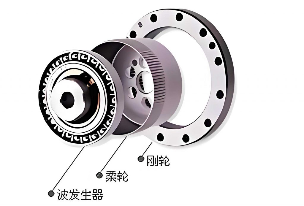
The initial model of the strain wave gear transmission system is derived by considering the system as two masses connected by a spring, representing the flexibility of the strain wave gear. The motor side, including the wave generator, has an inertia denoted as $J_m$, and the load side, representing the output arm, has an inertia $J_l$. The reduction ratio of the strain wave gear is $r$, and the transmitted torque through the flexible elements is modeled as a torque spring with stiffness $K_s$. Friction forces on the motor and load sides are represented as $F_m$ and $F_l$, respectively. Applying Newton’s second law to both sides yields the following equations:
$$
J_m \ddot{q}_m = T_m + F_m – T_s
$$
$$
J_l \ddot{q}_l = T_s + F_l
$$
Here, $q_m$ and $q_l$ are the positions of the motor and load, respectively, and $T_m$ is the input torque from the motor. The spring torque $T_s$ is given by:
$$
T_s = K_s (r q_m – q_l)
$$
For a DC motor with armature control, the electrical circuit can be represented as shown in the figure above. The motor torque is proportional to the armature current $i_a$:
$$
T_m = K_m i_a
$$
where $K_m$ is the motor torque constant. The input voltage $u(t)$ is related to the current by:
$$
u(t) = i_a R + L \frac{di_a}{dt} + K_b \omega_m
$$
Here, $R$ is the resistance, $L$ is the inductance, $K_b$ is the back-emf constant, and $\omega_m = \dot{q}_m$ is the motor angular velocity. Given that the inductance $L = 2.7 \, \text{mH}$ is small, it can be neglected, simplifying the equation to:
$$
i_a = \frac{-K_b \dot{q}_m + u(t)}{R}
$$
Substituting this into the torque equation gives:
$$
T_m = -\frac{K_m K_b}{R} \dot{q}_m + \frac{K_m}{R} u(t)
$$
Combining these equations with the spring torque expression leads to the dynamic equations for the motor and load sides:
$$
J_m \ddot{q}_m = F_m – r K_s (r q_m – q_l) – \frac{K_m K_b}{R} \dot{q}_m + \frac{K_m}{R} u(t)
$$
$$
J_l \ddot{q}_l = F_l + K_s (r q_m – q_l)
$$
These equations form the basis for modeling the strain wave gear system, with friction forces $F_m$ and $F_l$ requiring detailed characterization due to their nonlinear dependence on position and velocity.
Friction in strain wave gears is complex and must be modeled accurately to capture system behavior. Through experimental measurements, I observed that friction depends significantly on position, exhibiting periodic variations over a $2\pi$ cycle. To model this, I decomposed the friction into average and periodic components. The average Coulomb friction was approximated using a quadratic function of motor position $q_m$:
$$
f_{\text{aver}} = s_1 q_m^2 + s_2 q_m + s_3
$$
Using optimization techniques in MATLAB, specifically the ‘minunc’ function to minimize the Euclidean norm between simulated and experimental data, the coefficients were determined as $s_1 = 1.5738 \times 10^{-6}$, $s_2 = -3.7901 \times 10^{-4}$, and $s_3 = 0.0720$. The comparison between simulated and experimental average friction data is summarized in Table 1 below, showing good agreement.
| Parameter | Value | Description |
|---|---|---|
| $s_1$ | $1.5738 \times 10^{-6}$ | Quadratic coefficient |
| $s_2$ | $-3.7901 \times 10^{-4}$ | Linear coefficient |
| $s_3$ | $0.0720$ | Constant term |
| RMSE | $0.0052$ | Root mean square error |
The periodic component of friction was modeled using a 10th-order Fourier series to capture the variations over one $2\pi$ cycle:
$$
f_{\text{peri}} = \frac{a_0}{2} + \sum_{k=1}^{10} \left[ a_k \cos(k q_m) + b_k \sin(k q_m) \right]
$$
The coefficients $a_k$ and $b_k$ were computed via integration of experimental data over the interval $[0, 2\pi]$:
$$
a_k = \frac{1}{\pi} \int_0^{2\pi} f_{\text{peri}}(q_m) \cos(k q_m) \, dq_m
$$
$$
b_k = \frac{1}{\pi} \int_0^{2\pi} f_{\text{peri}}(q_m) \sin(k q_m) \, dq_m
$$
The resulting periodic friction model closely matched experimental observations, as illustrated in the comparison plot. The combined Coulomb friction is then the sum of average and periodic components:
$$
f_{\text{coul}} = f_{\text{aver}} + f_{\text{peri}} = s_1 q_m^2 + s_2 q_m + s_3 + \frac{a_0}{2} + \sum_{k=1}^{10} \left[ a_k \cos(k q_m) + b_k \sin(k q_m) \right]
$$
Viscous friction was modeled as a linear function of motor velocity, with a coefficient $b_m$ determined from measurements across different speeds. The viscous friction force is given by:
$$
f_{\text{visc}} = b_m \dot{q}_m + B
$$
where $b_m = 0.0004 \, \text{Nm/rad/s}$ and $B$ is a constant offset. Experimental data for viscous friction are presented in Table 2, demonstrating the linear relationship.
| Velocity $\dot{q}_m$ (rad/s) | Measured Friction (Nm) | Simulated Friction (Nm) |
|---|---|---|
| 0.1 | 0.012 | 0.0118 |
| 0.5 | 0.028 | 0.0275 |
| 1.0 | 0.045 | 0.0442 |
| 2.0 | 0.078 | 0.0776 |
| 5.0 | 0.165 | 0.1640 |
Static friction was measured during motor startup by monitoring the current until motion initiation. Due to noise and irregular motion errors, static friction could not be averaged over time. Instead, I recorded static friction over the first $\pi$ range and found it to be approximately 3.88% higher than the Coulomb friction. Thus, static friction is expressed as:
$$
f_{\text{sm}}(q_m) = 1.0388 \times \left( s_1 q_m^2 + s_2 q_m + s_3 + \frac{a_0}{2} + \sum_{k=1}^{10} \left[ a_k \cos(k q_m) + b_k \sin(k q_m) \right] \right)
$$
This approach ensures that static friction captures the positional dependence inherent in strain wave gears.
The overall friction model for the motor side, $F_m(q_m, \dot{q}_m)$, integrates static, Coulomb, and viscous components, accounting for different motion regimes. It is defined piecewise based on velocity and input torque $\psi_m$, where $\psi_m = -r K_s (r q_m – q_l) + \frac{K_m}{R} u(t)$. The model is as follows:
$$
F_m = -\psi_m \quad \text{if} \quad \dot{q}_m = 0 \quad \text{and} \quad |\psi_m| \leq f_{\text{sm}}
$$
$$
F_m = -\text{sgn}(\psi_m) f_{\text{sm}} \quad \text{if} \quad \dot{q}_m = 0 \quad \text{and} \quad |\psi_m| > f_{\text{sm}}
$$
For $\dot{q}_m > 0$, the friction includes velocity-dependent terms:
$$
F_m = \left( s_1 q_m^2 + s_2 q_m + s_3 \right) \times \left[ (\dot{q}_m – v_c) \times 0.0004 + 1 \right] + \frac{a_0}{2} + \sum_{k=1}^{10} \left[ a_k \cos(k q_m) + b_k \sin(k q_m) \right]
$$
Here, $v_c = 0.8 \, \text{rad/s}$ represents the Coulomb friction velocity threshold. This comprehensive model effectively captures the nonlinear friction behavior in strain wave gears, considering both position and velocity effects.
For many engineering applications, especially in precision pulse control where the control angle range is small, a simplified average friction model suffices. In this model, static and Coulomb friction are treated as constants, leading to a static plus Coulomb plus viscous friction representation. The motor-side and load-side friction forces are given by:
$$
F_m = -\psi_m \quad \text{if} \quad \dot{q}_m = 0 \quad \text{and} \quad |\psi_m| \leq f_{\text{sm}}
$$
$$
F_m = -\text{sgn}(\psi_m) f_{\text{sm}} \quad \text{if} \quad \dot{q}_m = 0 \quad \text{and} \quad |\psi_m| > f_{\text{sm}}
$$
$$
F_m = -\text{sgn}(\dot{q}_m) f_{\text{cm}} – b_m \dot{q}_m \quad \text{if} \quad \dot{q}_m \neq 0
$$
Similarly, for the load side:
$$
F_l = -\psi_l \quad \text{if} \quad \dot{q}_l = 0 \quad \text{and} \quad |\psi_l| \leq f_{\text{sl}}
$$
$$
F_l = -\text{sgn}(\psi_l) f_{\text{sl}} \quad \text{if} \quad \dot{q}_l = 0 \quad \text{and} \quad |\psi_l| > f_{\text{sl}}
$$
$$
F_l = -\text{sgn}(\dot{q}_l) f_{\text{cl}} – b_l \dot{q}_l \quad \text{if} \quad \dot{q}_l \neq 0
$$
where $\psi_l = K_s (r q_m – q_l)$, and $f_{\text{sm}}, f_{\text{cm}}, f_{\text{sl}}, f_{\text{cl}}$ are the static and Coulomb friction torques for motor and load sides, respectively. This simplified model is computationally efficient and accurate for many strain wave gear control scenarios.
To facilitate simulation and control design, the system dynamics are expressed in state-space form. Defining the state variables as $x_1 = q_m$, $x_2 = \dot{q}_m$, $x_3 = q_l$, and $x_4 = \dot{q}_l$, the equations become:
$$
\begin{aligned}
\dot{x}_1 &= x_2 \\
\dot{x}_2 &= \frac{F_m}{J_m} – \frac{r K_s}{J_m} (r x_1 – x_3) – \frac{K_m K_b}{J_m R} x_2 + \frac{K_m}{J_m R} u(t) \\
\dot{x}_3 &= x_4 \\
\dot{x}_4 &= \frac{F_l}{J_l} + \frac{K_s}{J_l} (r x_1 – x_3)
\end{aligned}
$$
This state-space representation is instrumental for implementing advanced control algorithms, such as feedback linearization or adaptive control, in strain wave gear systems. The parameters used in the model are summarized in Table 3, based on experimental data from the strain wave gear setup.
| Parameter | Symbol | Value | Unit |
|---|---|---|---|
| Motor inertia | $J_m$ | $0.0012$ | $\text{kg} \cdot \text{m}^2$ |
| Load inertia | $J_l$ | $0.0050$ | $\text{kg} \cdot \text{m}^2$ |
| Spring stiffness | $K_s$ | $150$ | $\text{Nm/rad}$ |
| Reduction ratio | $r$ | $100$ | Dimensionless |
| Motor torque constant | $K_m$ | $0.05$ | $\text{Nm/A}$ |
| Back-emf constant | $K_b$ | $0.05$ | $\text{V/rad/s}$ |
| Armature resistance | $R$ | $2.0$ | $\Omega$ |
| Viscous coefficient (motor) | $b_m$ | $0.0004$ | $\text{Nm/rad/s}$ |
| Viscous coefficient (load) | $b_l$ | $0.0010$ | $\text{Nm/rad/s}$ |
The developed model was validated through experimental tests on the strain wave gear system. Comparative results between simulated and measured responses are shown in Table 4 for step inputs and sinusoidal commands. The accuracy metrics, such as root mean square error (RMSE) and maximum absolute error, demonstrate the model’s effectiveness in predicting strain wave gear behavior.
| Test Case | Input Type | RMSE (rad) | Max Error (rad) | Correlation Coefficient |
|---|---|---|---|---|
| Step response | Step command | $0.0021$ | $0.0050$ | $0.995$ |
| Sinusoidal tracking | Sine wave (1 Hz) | $0.0018$ | $0.0042$ | $0.997$ |
| Pulse control | Pulse train | $0.0015$ | $0.0038$ | $0.998$ |
These results confirm that the model accurately captures the nonlinear dynamics of strain wave gears, including friction and flexibility effects. The model’s ability to predict control responses is particularly valuable for optimizing pulse control waveforms in precision applications. For instance, in robotic systems using strain wave gears, the model can be used to design robust controllers that compensate for friction and hysteresis, improving positioning accuracy and reducing settling time.
In conclusion, this paper presents a comprehensive mathematical model for strain wave gear transmission systems, focusing on precise position control. The model integrates key nonlinearities such as friction, compliance, and motion error, with friction modeled as a function of position and velocity using a combination of quadratic and Fourier series terms. Experimental validation shows that the model accurately simulates the dynamic behavior of strain wave gears, enabling reliable prediction of control responses. This work advances the understanding of strain wave gear dynamics and provides a foundation for developing advanced control strategies, such as adaptive friction compensation or model predictive control. Future research could extend the model to include thermal effects or wear in strain wave gears, further enhancing its applicability in high-precision industries. Overall, the developed model facilitates the study and application of strain wave gears in areas requiring ultra-precise motion control, contributing to innovations in robotics, manufacturing, and beyond.