
In the field of robotics, the development of a dexterous robotic hand has been a significant focus, particularly for applications requiring high precision and flexibility, such as in medical massage therapy. The study of inverse dynamics problems aims to enhance the stability and control accuracy of robotic systems, enabling optimal control of the dexterous robotic hand for improved dynamic performance and metrics. This article explores the dynamics of a specific dexterous robotic hand, the Shadow dexterous hand, by establishing a dynamic model based on kinematic research conclusions. The analysis covers finger link dynamics, tendon transmission system dynamics, and actuator dynamics, ultimately deriving the single-finger dynamics equation to provide a theoretical foundation for simulation and practical application.
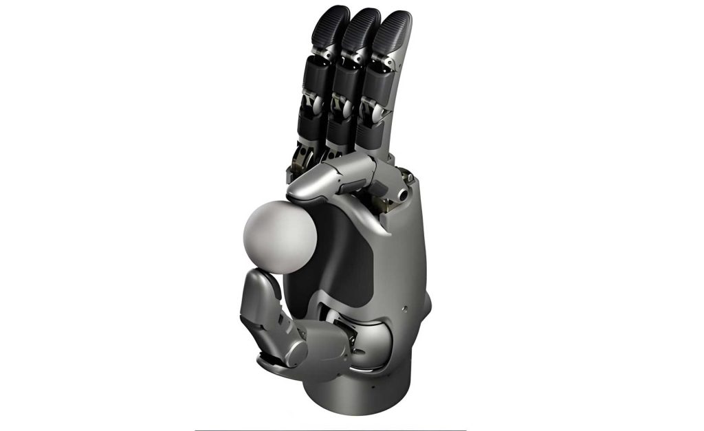
The dexterous robotic hand in question is characterized by its anthropomorphic design, with 24 joints and 20 degrees of freedom. The thumb features a 5-joint structure with 5 degrees of freedom, while the index, middle, and ring fingers have 4-joint structures with 3 degrees of freedom each. The little finger, similar to the middle finger, includes an additional metacarpal joint, totaling 4 degrees of freedom. This dexterous robotic hand is driven by 40 pneumatic muscle actuators (PMAs) using tendon transmission, where forces and moments are transmitted from joints to fingertips. Integrated sensors, such as joint position sensors, pressure sensors, and fingertip tactile array sensors, facilitate precise control. The focus here is on the dynamics of a single finger, using the middle finger as an example due to its representative structure.
Dynamics analysis of the dexterous robotic hand involves studying the relationship between the torques required to drive finger joints and the angular displacement, velocity, and acceleration during motion. The dynamic model for the dexterous robotic hand comprises three components: finger link dynamics, tendon transmission system dynamics, and actuator dynamics. Each component contributes to the overall performance of the dexterous robotic hand, and their integration is crucial for accurate control.
First, the finger link dynamics of the dexterous robotic hand are analyzed using the Newton-Euler method. This iterative algorithm involves outward iteration from link 1 to link 4 to compute linear and angular velocities and accelerations, followed by inward iteration from link 4 to link 1 to determine joint driving torques. The closed-form dynamics equation for the middle finger of the dexterous robotic hand is given by:
$$ \tau = D(q) \ddot{q} + h(q, \dot{q}) + G(q) $$
where \(\tau\) is the joint torque vector, \(q\) is the joint angular displacement vector, \(\dot{q}\) is the joint angular velocity vector, \(\ddot{q}\) is the joint angular acceleration vector, \(D(q)\) is the inertia matrix (a 4×4 positive definite matrix), \(h(q, \dot{q})\) represents centrifugal and Coriolis forces, and \(G(q)\) is the gravity vector. Friction effects, including viscous friction \(\tau_v = v \dot{\theta}\) and Coulomb friction \(\tau_\mu = N_f \mu \text{sgn}(\dot{\theta})\), are incorporated as \(\tau_f\), leading to the modified equation:
$$ \tau = D(q) \ddot{q} + h(q, \dot{q}) + G(q) + \tau_f $$
This equation forms the basis for understanding the inertial and gravitational forces in the dexterous robotic hand.
Second, the tendon transmission system dynamics of the dexterous robotic hand are examined. Tendons in the dexterous robotic hand are lightweight, low-inertia, and low-friction, simplifying the model. Each tendon’s displacement \(h_j\) is a linear function of joint angles:
$$ h_j = h_{0j} \pm r_1 \theta_1 \pm r_2 \theta_2 \ldots \pm r_i \theta_i \ldots r_n \theta_n $$
where \(h_{0j}\) is the initial displacement, \(r_i\) is the pulley radius, and \(\theta_i\) is the joint angle. Using energy conservation, the work done by tendons equals the work done by the finger, yielding:
$$ \tau^T \Delta q = f^T \Delta h $$
Here, \(f\) is the tendon tension vector, and \(\Delta h\) is the tendon displacement change vector. Defining matrix \(P = \frac{\partial h^T}{\partial q}\), we derive:
$$ \tau = P f $$
and
$$ \Delta h = P^T \Delta q $$
These equations relate joint torques to tendon tensions in the dexterous robotic hand, essential for control design.
Third, the actuator dynamics of the dexterous robotic hand are analyzed using the McKibben-type PMA model. The PMA consists of an inner rubber tube and an outer braided mesh, generating axial contraction force upon inflation. The force \(f_i\) for the i-th PMA is modeled as:
$$ f_i = p_a \frac{\pi D_0^2}{4 \sin^2 \theta_0} \left[ 3 \frac{L_i^2}{L_{0i}^2} \cos^2 \theta_0 – 1 \right] $$
where \(p_a\) is the inflation pressure, \(D_0\) is the initial diameter, \(\theta_0\) is the initial fiber angle, \(L_{0i}\) is the initial length, and \(L_i\) is the current length. Assuming inelastic tendons, the length change relates to tendon displacement: \(L = L_0 – \Delta h = L_0 – P^T q\). This model captures the pneumatic actuation characteristics of the dexterous robotic hand.
Integrating these components, the overall single-finger dynamics equation for the dexterous robotic hand is derived. From robotics statics, the relationship between joint torques and external forces is \(\tau = J^T \cdot f_{\text{ext}}\), where \(J\) is the Jacobian matrix and \(f_{\text{ext}}\) is the external contact force vector. Combining this with the previous equations, we obtain:
$$ D(q) \ddot{q} + h(q, \dot{q}) + G(q) + \tau_f = P f – J^T \cdot f_{\text{ext}} $$
This equation, along with \(L = L_0 – P^T q\), describes the interplay between joint motion parameters, PMA contractions, and external forces in the dexterous robotic hand. It serves as a foundation for real-time control and simulation of the dexterous robotic hand.
To further elucidate the dynamics, key parameters and equations are summarized in tables. For instance, Table 1 outlines the notation used in the dynamics model of the dexterous robotic hand.
| Symbol | Description | Unit |
|---|---|---|
| \(\tau\) | Joint torque vector | Nm |
| \(q\) | Joint angular displacement vector | rad |
| \(\dot{q}\) | Joint angular velocity vector | rad/s |
| \(\ddot{q}\) | Joint angular acceleration vector | rad/s² |
| \(D(q)\) | Inertia matrix | kg·m² |
| \(h(q, \dot{q})\) | Centrifugal/Coriolis force vector | N |
| \(G(q)\) | Gravity vector | N |
| \(\tau_f\) | Friction torque vector | Nm |
| \(f\) | Tendon tension vector | N |
| \(P\) | Tendon displacement Jacobian | m/rad |
| \(J\) | Finger Jacobian matrix | — |
| \(f_{\text{ext}}\) | External force vector | N |
| \(L\) | PMA length vector | m |
| \(p_a\) | Inflation pressure | Pa |
Additionally, Table 2 provides typical parameter values for the dexterous robotic hand, based on the Shadow hand design.
| Parameter | Value | Description |
|---|---|---|
| Number of joints | 24 | Total joints in the dexterous robotic hand |
| Degrees of freedom | 20 | Independent motions of the dexterous robotic hand |
| PMA count | 40 | Actuators driving the dexterous robotic hand |
| Tendon stiffness | High | Assumed for simplification in the dexterous robotic hand |
| Friction coefficients | \(v = 0.01\), \(\mu = 0.1\) | Typical values for the dexterous robotic hand |
| Initial PMA diameter \(D_0\) | 10 mm | For McKibben-type actuators in the dexterous robotic hand |
| Initial fiber angle \(\theta_0\) | 20° | For PMA model in the dexterous robotic hand |
The dynamics of the dexterous robotic hand can be further analyzed through simulation scenarios. For example, consider a trajectory tracking task where the middle finger of the dexterous robotic hand moves from an initial to a final position. The joint angles, velocities, and accelerations are specified, and the required torques are computed using the dynamics equation. This process involves solving the inverse dynamics problem for the dexterous robotic hand, which is crucial for control system design. The equations are implemented in a step-by-step manner, as outlined below.
Step 1: Define the trajectory for the dexterous robotic hand. Let \(q_d(t)\) be the desired joint angle vector over time \(t\). For simplicity, a polynomial trajectory is often used:
$$ q_d(t) = a_0 + a_1 t + a_2 t^2 + a_3 t^3 $$
where coefficients \(a_i\) are determined from boundary conditions. This ensures smooth motion for the dexterous robotic hand.
Step 2: Compute derivatives for the dexterous robotic hand:
$$ \dot{q}_d(t) = a_1 + 2a_2 t + 3a_3 t^2 $$
$$ \ddot{q}_d(t) = 2a_2 + 6a_3 t $$
These represent the desired velocity and acceleration profiles for the dexterous robotic hand.
Step 3: Calculate the inertia matrix \(D(q)\) for the dexterous robotic hand. For a four-link finger, \(D(q)\) is a 4×4 matrix with elements dependent on link masses \(m_i\), lengths \(l_i\), and inertia tensors. Using standard robotic formulations, \(D(q)\) can be expressed as:
$$ D(q) = \begin{bmatrix} D_{11} & D_{12} & D_{13} & D_{14} \\ D_{21} & D_{22} & D_{23} & D_{24} \\ D_{31} & D_{32} & D_{33} & D_{34} \\ D_{41} & D_{42} & D_{43} & D_{44} \end{bmatrix} $$
where each \(D_{ij}\) is a function of \(q\). For instance, \(D_{11}\) might include terms like \(m_1 l_{c1}^2 + I_1 + m_2 l_1^2 + \ldots\), with \(l_{ci}\) as the center of mass distance. This matrix captures the mass distribution of the dexterous robotic hand.
Step 4: Determine the centrifugal and Coriolis vector \(h(q, \dot{q})\) for the dexterous robotic hand. This vector is derived from the Christoffel symbols based on \(D(q)\):
$$ h_i(q, \dot{q}) = \sum_{j=1}^{4} \sum_{k=1}^{4} c_{ijk} \dot{q}_j \dot{q}_k $$
where \(c_{ijk} = \frac{1}{2} \left( \frac{\partial D_{ij}}{\partial q_k} + \frac{\partial D_{ik}}{\partial q_j} – \frac{\partial D_{jk}}{\partial q_i} \right)\). These terms account for velocity-dependent forces in the dexterous robotic hand.
Step 5: Compute the gravity vector \(G(q)\) for the dexterous robotic hand. For a finger with links in a gravitational field, \(G(q) = \frac{\partial U}{\partial q}\), where \(U\) is the potential energy. If gravity acts along the negative z-axis, then:
$$ G_i(q) = \sum_{j=1}^{4} m_j g \, z_{cj}(q) $$
with \(g\) as gravitational acceleration and \(z_{cj}\) as the z-coordinate of the center of mass of link j. This reflects the weight effects on the dexterous robotic hand.
Step 6: Include friction torques \(\tau_f\) for the dexterous robotic hand. Using the viscous and Coulomb models:
$$ \tau_{fi} = v \dot{q}_i + N_f \mu \text{sgn}(\dot{q}_i) $$
where \(N_f\) is the normal force, often estimated from contact conditions. Friction can significantly impact the dexterous robotic hand’s performance.
Step 7: Solve for tendon tensions \(f\) in the dexterous robotic hand. From \(\tau = P f\), and given \(P\) based on tendon routing, we have:
$$ f = P^{\dagger} \tau $$
where \(P^{\dagger}\) is the pseudoinverse of \(P\), since \(P\) may not be square. This ensures feasible tendon forces for the dexterous robotic hand.
Step 8: Relate to PMA forces for the dexterous robotic hand. Using the PMA model, the inflation pressure \(p_a\) can be adjusted to achieve the desired \(f\). For each PMA, from \(f_i = p_a \frac{\pi D_0^2}{4 \sin^2 \theta_0} \left[ 3 \frac{L_i^2}{L_{0i}^2} \cos^2 \theta_0 – 1 \right]\), we can solve for \(p_a\) given \(L_i = L_{0i} – \Delta h_i\). This closes the loop for controlling the dexterous robotic hand.
These steps illustrate the computational framework for dynamics analysis of the dexterous robotic hand. In practice, numerical methods are employed for real-time implementation. The complexity arises from the coupling between links, tendons, and actuators in the dexterous robotic hand, but the derived equations provide a systematic approach.
Furthermore, the dynamics of the dexterous robotic hand can be validated through experiments or simulations. For instance, using software like MATLAB or ROS, one can simulate the motion of the dexterous robotic hand under various loads. The dynamics equation can be discretized for simulation, such as via the Euler method:
$$ \ddot{q}_{k+1} = D^{-1}(q_k) \left[ \tau_k – h(q_k, \dot{q}_k) – G(q_k) – \tau_{f,k} \right] $$
$$ \dot{q}_{k+1} = \dot{q}_k + \ddot{q}_k \Delta t $$
$$ q_{k+1} = q_k + \dot{q}_k \Delta t $$
where \(k\) is the time step and \(\Delta t\) is the sampling time. This allows for dynamic response analysis of the dexterous robotic hand.
Another aspect is the optimization of the dexterous robotic hand’s design based on dynamics. Parameters like link lengths, masses, and tendon routing can be tuned to minimize energy consumption or maximize speed. For example, the inertia matrix \(D(q)\) influences the torque requirements; reducing link masses can enhance the agility of the dexterous robotic hand. Similarly, tendon stiffness affects force transmission; higher stiffness improves precision but may increase control complexity. These trade-offs are critical for advanced dexterous robotic hand applications.
In terms of control strategies for the dexterous robotic hand, the dynamics equation enables model-based controllers such as computed torque control. The control law for the dexterous robotic hand can be:
$$ \tau = D(q) \left[ \ddot{q}_d + K_v (\dot{q}_d – \dot{q}) + K_p (q_d – q) \right] + h(q, \dot{q}) + G(q) $$
where \(K_p\) and \(K_v\) are gain matrices. This compensates for nonlinearities and disturbances in the dexterous robotic hand. Additionally, adaptive control can be used to handle parameter uncertainties in the dexterous robotic hand, such as varying payloads.
The tendon transmission system in the dexterous robotic hand also warrants detailed analysis. The matrix \(P\) encodes the tendon routing geometry. For the middle finger with 6 tendons controlling 3 independent degrees of freedom (plus coupling), \(P\) is a 4×6 matrix. A sample \(P\) matrix might be:
$$ P = \begin{bmatrix} r_1 & -r_1 & 0 & 0 & 0 & 0 \\ 0 & 0 & r_2 & -r_2 & 0 & 0 \\ 0 & 0 & 0 & 0 & r_3 & -r_3 \\ 0 & 0 & 0 & 0 & r_4 & -r_4 \end{bmatrix} $$
where \(r_i\) are pulley radii. This shows that tendons 1 and 2 control joint 1, tendons 3 and 4 control joint 2, and tendons 5 and 6 control joints 3 and 4 in a coupled manner. This design reduces actuator count in the dexterous robotic hand.
The PMA dynamics for the dexterous robotic hand can be extended to include thermodynamic effects. The force model might incorporate temperature and hysteresis, but for control purposes, a simplified version suffices. The length-force relationship is pivotal for the dexterous robotic hand’s actuation. Moreover, the PMAs exhibit nonlinear behavior, which can be linearized around operating points for simpler control of the dexterous robotic hand.
To summarize the key equations for the dexterous robotic hand, we list them below:
1. Finger link dynamics: $$ \tau = D(q) \ddot{q} + h(q, \dot{q}) + G(q) + \tau_f $$
2. Tendon transmission: $$ \tau = P f, \quad \Delta h = P^T \Delta q $$
3. PMA force model: $$ f_i = p_a \frac{\pi D_0^2}{4 \sin^2 \theta_0} \left[ 3 \frac{L_i^2}{L_{0i}^2} \cos^2 \theta_0 – 1 \right] $$
4. Length relation: $$ L = L_0 – P^T q $$
5. Overall dynamics: $$ D(q) \ddot{q} + h(q, \dot{q}) + G(q) + \tau_f = P f – J^T \cdot f_{\text{ext}} $$
These equations form a comprehensive model for the dexterous robotic hand. For practical implementation, parameter identification is necessary. Experimental data from the dexterous robotic hand can be used to estimate \(D(q)\), \(h(q, \dot{q})\), and friction coefficients via system identification techniques.
In conclusion, the dynamics analysis of the dexterous robotic hand provides insights into the torque-motion relationships essential for control. The integration of link, tendon, and actuator dynamics enables accurate modeling of the dexterous robotic hand. Future work may involve extending this to multi-finger coordination or incorporating tactile feedback for interactive tasks. The dexterous robotic hand’s potential in fields like rehabilitation, prosthetics, and industrial automation hinges on such dynamical understanding. Ultimately, this research contributes to the advancement of robotic manipulation, making the dexterous robotic hand more adaptive and efficient.