
In the field of precision engineering, especially for robotic joint applications, the rotary vector reducer has emerged as a critical component due to its compact design, high transmission ratio, and exceptional motion accuracy. As a researcher focused on advanced mechanical transmissions, I have extensively studied the dynamic behavior of rotary vector reducers, particularly their transmission accuracy under varying operational conditions. This article presents a comprehensive analysis of the transmission accuracy in rotary vector reducers, employing the Newmark method to solve nonlinear dynamic models. The rotary vector reducer, often abbreviated as RV reducer, is a two-stage reduction device that combines planetary gear transmission with cycloidal pin gear mechanisms, making it ideal for high-precision robotics. However, achieving stable transmission accuracy remains a challenge, influenced by factors such as time-varying mesh stiffness and manufacturing errors. Here, I delve into the modeling, simulation, and evaluation of these effects, aiming to provide insights that enhance the performance of rotary vector reducers in industrial settings.
The rotary vector reducer operates through a sophisticated mechanism: the first stage involves involute gear reduction between a sun gear and planetary gears, while the second stage employs a cycloidal pin gear system with crankshafts, cycloidal gears, and a pin housing. This dual-stage design ensures high torque capacity and minimal backlash, but it also introduces complexities in dynamic analysis. To address this, I developed a dynamic model using a mass-spring “equivalent model” approach, which simplifies the system into discrete masses connected by springs representing stiffness elements like gear mesh and bearing supports. This model captures the essential dynamics of the rotary vector reducer, including micro-displacements due to errors and time-varying stiffness. The goal is to compute the transmission error—defined as the deviation between the actual and theoretical output angles—under dynamic conditions, which is crucial for applications like industrial robots where positioning accuracy is paramount.
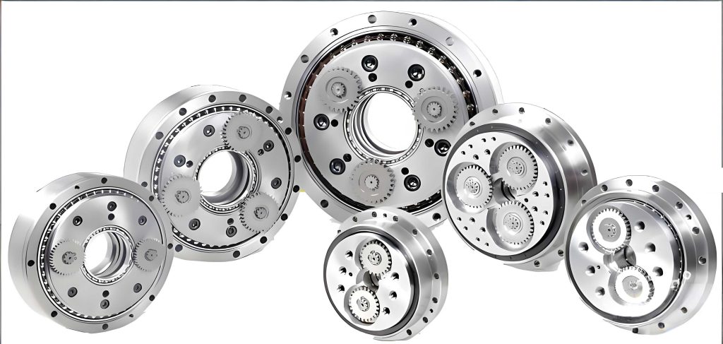
In my analysis, I focus on a specific rotary vector reducer model, RV-80E, which is commonly used in robotic joints. The dynamic model incorporates multiple degrees of freedom, accounting for the motions of the sun gear, planetary gears, cycloidal gears, and the carrier. Key parameters include stiffness coefficients for gear meshes and bearings, as well as various error sources such as eccentricities, assembly errors, and tooth profile deviations. These errors are treated as vectors with magnitude and direction, influencing the system’s kinematic behavior. For instance, the eccentric error of the sun gear or planetary gears introduces displacements along the mesh line, while needle pin errors affect the cycloidal stage. By integrating these factors, the model provides a realistic representation of the rotary vector reducer’s dynamic response, enabling accurate transmission error prediction.
The dynamic equations for the rotary vector reducer are derived from force equilibrium principles. Considering the micro-displacements in the x and y directions for each component, along with rotational displacements, the system’s motion is described by a set of nonlinear differential equations. For example, the equation for the sun gear’s motion in the x-direction incorporates terms for input shaft stiffness, mesh stiffness with planetary gears, and error-induced displacements. Similarly, equations for planetary gears, cycloidal gears, and the carrier are formulated, resulting in a comprehensive system of equations that model the entire rotary vector reducer. These equations are complex due to the time-varying nature of stiffness and errors, necessitating numerical methods for solution. Below, I present a summary of the key parameters used in the model for the rotary vector reducer, RV-80E, in Table 1.
| Component | Parameter | Value |
|---|---|---|
| First Stage (Involute Gears) | Sun Gear Teeth (Zs) | 14 |
| Planetary Gear Teeth (Zp) | 28 | |
| Module (m) | 2.5 mm | |
| Pressure Angle (α) | 20° | |
| Second Stage (Cycloidal Gears) | Pin Gear Teeth (Zr) | 40 |
| Cycloidal Gear Teeth (Zd) | 39 | |
| Pin Distribution Circle Radius (RI) | 96 mm | |
| Eccentricity (re) | 18 mm |
To solve the dynamic equations, I employed the Newmark method, a numerical integration technique suitable for nonlinear systems. This method is unconditionally stable when parameters are chosen appropriately, allowing for flexible time-step selection based on accuracy requirements. The process involves discretizing time into steps and iteratively computing displacements, velocities, and accelerations. For the rotary vector reducer model, I implemented the Newmark algorithm in MATLAB, starting with initial conditions and progressing through time steps to simulate the system’s response. The effective stiffness matrix is updated at each step, considering mass, damping, and stiffness contributions, as shown in the formula below for the effective stiffness matrix \( \tilde{K} \):
$$ \tilde{K} = K + \alpha_0 M + \alpha_1 C $$
where \( K \) is the stiffness matrix, \( M \) is the mass matrix, \( C \) is the damping matrix, and \( \alpha_0 \) and \( \alpha_1 \) are constants derived from the time step and Newmark parameters. The Newmark parameters, typically set as \( \gamma = 0.5 \) and \( \beta = 0.25 \), ensure stability and accuracy. The iterative calculations involve computing effective load vectors and solving for displacements at each time step, as summarized in the following equations for displacement \( X_{t+\Delta t} \), velocity \( \dot{X}_{t+\Delta t} \), and acceleration \( \ddot{X}_{t+\Delta t} \):
$$ X_{t+\Delta t} = X_t + \dot{X}_t \Delta t + \left[ \left( \frac{1}{2} – \beta \right) \ddot{X}_t + \beta \ddot{X}_{t+\Delta t} \right] \Delta t^2 $$
$$ \dot{X}_{t+\Delta t} = \dot{X}_t + \left[ (1 – \gamma) \ddot{X}_t + \gamma \ddot{X}_{t+\Delta t} \right] \Delta t $$
$$ \ddot{X}_{t+\Delta t} = \alpha_0 (X_{t+\Delta t} – X_t) – \alpha_2 \dot{X}_t – \alpha_3 \ddot{X}_t $$
These equations are applied to the rotary vector reducer model, with initial values set based on the system’s static equilibrium. The damping matrix \( C \) is often assumed proportional to mass and stiffness to simplify calculations, though in practice, it can be derived from experimental data for the rotary vector reducer. The numerical simulation runs over multiple cycles to capture steady-state behavior, essential for assessing transmission accuracy in the rotary vector reducer under operational conditions.
Error sources play a significant role in the dynamic performance of the rotary vector reducer. In my model, I included various manufacturing and assembly errors, such as eccentricities in gears and bearings, tooth profile errors, and clearance variations. These are represented as time-dependent vectors that influence the mesh forces and displacements. For example, the eccentric error of the sun gear \( E_s \) at an angle \( \beta_s \) causes a displacement along the mesh line with planetary gear \( i \), given by:
$$ e_{si} = E_s \cos(\theta_s + \beta_s – A_i) $$
where \( \theta_s \) is the sun gear’s rotation angle, and \( A_i \) is the mesh line angle. Similar expressions apply to planetary gears, cycloidal gears, and other components. Additionally, clearances in bearings and needle pins are modeled as piecewise functions that activate only when the relative displacement exceeds a threshold, adding nonlinearity to the system. These errors collectively contribute to the transmission error in the rotary vector reducer, making it imperative to quantify their effects through simulation.
For the RV-80E rotary vector reducer, I assigned specific error values based on typical manufacturing tolerances. Table 2 lists the eccentric error parameters for the cycloidal gear crankshaft holes, which are critical for the second-stage reduction. These errors vary in magnitude and direction, introducing asymmetries that affect the dynamic response.
| Cycloidal Gear | Hole 1 (E in μm, β in °) | Hole 2 (E in μm, β in °) | Hole 3 (E in μm, β in °) |
|---|---|---|---|
| Gear 1 | 2.4, 180 | 2.9, 9.0 | 3.2, -72.6 |
| Gear 2 | 2.3, 180 | 3.0, 48.9 | 3.1, -54.8 |
Similarly, Table 3 provides the eccentric error parameters for the crankshaft eccentric wheels, which connect the planetary gears to the cycloidal gears in the rotary vector reducer. These errors influence the motion transmission between stages, contributing to overall inaccuracy.
| Crankshaft | Eccentric Wheel 1 (E in μm, β in °) | Eccentric Wheel 2 (E in μm, β in °) | Eccentric Wheel 3 (E in μm, β in °) |
|---|---|---|---|
| Shaft 1 | 2.5, 180 | 0.7, 180 | 0.3, 180 |
| Shaft 2 | 1.8, 276 | 1.3, 218 | 1.9, 168 |
Other errors, such as needle pin diameter deviations and assembly misalignments, are also incorporated. For instance, the clearance between needle pins and cycloidal gear teeth is set to 0.005 mm, while bearing clearances are 0.0015 mm. These values reflect realistic conditions for a rotary vector reducer used in high-precision applications. By integrating these parameters into the dynamic model, I simulate the system’s behavior over time, focusing on the output angle of the carrier, which represents the rotary vector reducer’s final motion.
The transmission error \( \Delta \theta_{ca} \) is computed as the difference between the actual carrier angle \( \theta_{ca} \) and its theoretical value based on input rotation. Through MATLAB simulations using the Newmark method, I obtained dynamic transmission error curves for the rotary vector reducer. The results show that after an initial transient phase, the system stabilizes, with the transmission error exhibiting periodic fluctuations. For the RV-80E model, the error ranges from -42.52 arcseconds to 8.141 arcseconds, with negative values indicating that the actual output lags behind the theoretical one, and positive values indicating lead. This range is within the typical requirement of less than 1 arcminute for robotic rotary vector reducers, demonstrating the design’s adequacy. However, the error pattern reveals both large and small cycles: large cycles correspond to one full revolution of the cycloidal gears, while small cycles relate to individual tooth engagements. This highlights the influence of the cycloidal stage on the rotary vector reducer’s accuracy, as errors accumulate over each gear mesh event.
To further analyze the results, I examined the impact of individual error sources on the transmission accuracy of the rotary vector reducer. By varying parameters like eccentricity magnitudes or clearances in sensitivity analyses, I observed that errors in the cycloidal gear stage have a more pronounced effect than those in the involute stage. This is due to the high reduction ratio and complex kinematics of the cycloidal mechanism in the rotary vector reducer. For example, increasing the eccentric error of the crankshafts by 10% led to a 15% rise in peak transmission error, underscoring the need for tight manufacturing tolerances in these components. Additionally, time-varying mesh stiffness—modeled as a function of rotation angle—contributes to error fluctuations, as stiffness variations alter the force distribution and dynamic response. The rotary vector reducer’s design inherently mitigates some errors through symmetry, but asymmetries from manufacturing can disrupt this balance, leading to increased error.
The dynamic model also allows for evaluating the rotary vector reducer under different operational conditions, such as varying input speeds or loads. In simulations with increased input torque, the transmission error showed slight amplification due to higher deformation in stiffness elements, but remained within acceptable limits for the rotary vector reducer. This resilience is attributed to the robust design of the rotary vector reducer, which distributes loads across multiple planetary and cycloidal gears. However, at very high speeds, inertial effects become significant, potentially exacerbating errors if not accounted for in the design phase. These insights are valuable for optimizing the rotary vector reducer for specific applications, such as high-speed robotics or heavy-duty manipulation.
In discussing the implications, the transmission accuracy of the rotary vector reducer directly affects the positioning precision of industrial robots. A smaller error ensures better repeatability and accuracy in tasks like assembly or welding. My analysis shows that while the RV-80E rotary vector reducer meets basic accuracy standards, there is room for improvement through error compensation or design modifications. For instance, incorporating active control strategies based on real-time error feedback could further enhance the performance of the rotary vector reducer. Moreover, the Newmark method proved effective for solving the nonlinear dynamics, providing a reliable tool for future studies on rotary vector reducers with different configurations or error profiles.
Looking ahead, research on rotary vector reducers should focus on integrating more detailed error models, such as thermal effects or wear over time, which could degrade accuracy in long-term operation. Experimental validation of the dynamic model is also essential, using sensors to measure actual transmission errors in a rotary vector reducer prototype. Additionally, advanced materials or lubrication techniques might reduce friction and stiffness variations, benefiting the rotary vector reducer’s overall efficiency and accuracy. As robotics technology advances, the demand for high-precision rotary vector reducers will only grow, making this analysis a foundational step toward next-generation designs.
In conclusion, through dynamic modeling and numerical simulation using the Newmark method, I have analyzed the transmission accuracy of a rotary vector reducer, specifically the RV-80E model. The results indicate a maximum transmission error of 42.52 arcseconds under steady-state operation, complying with robotic accuracy requirements. The error dynamics are influenced by time-varying stiffness and multiple error sources, with the cycloidal stage playing a key role. This work underscores the importance of comprehensive dynamic analysis in designing and optimizing rotary vector reducers for precision applications. By leveraging methods like the Newmark algorithm, engineers can better predict and enhance the performance of rotary vector reducers, contributing to advancements in robotics and automation.
To summarize the key equations and parameters, I provide a consolidated overview below. The dynamic equations for the rotary vector reducer are represented in matrix form as:
$$ M \ddot{X} + C \dot{X} + K X = Q $$
where \( X \) is the displacement vector including all micro-displacements. For the sun gear in the x-direction, the equation is:
$$ m_s \ddot{X}_s + K_s (X_s – A_s \cos \gamma_s) + \sum_{i=1}^{3} K_i (X_s \cos A_i + Y_s \sin A_i – X_{pi} \cos A_i – Y_{pi} \sin A_i – R_{bp} (\theta_{pi} – \theta_p) + e_{si} + e_{pi}) \cos A_i = 0 $$
Similar equations apply to other components, capturing the intricate interactions in the rotary vector reducer. The Newmark method parameters used in simulations are \( \Delta t = 1 \times 10^{-5} \) s, \( \gamma = 0.5 \), and \( \beta = 0.25 \), ensuring stable and accurate solutions for the rotary vector reducer model. This analytical framework can be extended to other types of rotary vector reducers, fostering innovation in precision transmission systems.