
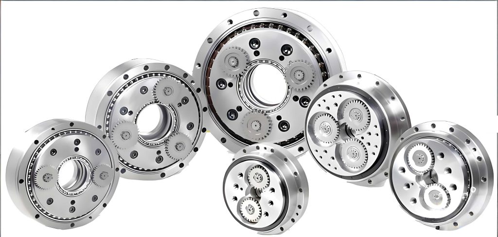
In modern industrial automation, rotary vector reducers serve as critical transmission components in robotics, offering high load-bearing capacity and precision. Their reliability directly impacts the operational efficiency and longevity of robotic systems. Traditional reliability assessment methods, often relying on time-consuming and costly life tests, have become inadequate for evaluating rotary vector reducers efficiently. Consequently, reliability evaluation based on performance degradation data has emerged as a promising alternative. In this article, I will explore a comprehensive approach to assessing the reliability of rotary vector reducers using transmission accuracy degradation data, incorporating mathematical models, statistical methods, and practical insights from accelerated testing.
The core idea behind performance degradation-based reliability assessment is to monitor key performance indicators over time, model their degradation trajectories, and predict failure times without waiting for complete failures. For rotary vector reducers, transmission error—defined as the deviation between the actual and theoretical output rotation angles under unidirectional input—is a vital performance metric. As the rotary vector reducer undergoes operational stresses, such as repeated reversals and impact loads, internal wear accumulates, leading to a gradual increase in transmission error and a decline in accuracy. This degradation ultimately affects the positioning precision of robots, making it a suitable candidate for reliability analysis.
To collect degradation data, I conducted accelerated degradation tests on rotary vector reducers. The testing involved subjecting the reducers to oscillatory motion under elevated loads to simulate real-world conditions while accelerating the degradation process. The test setup included a reciprocating swing test rig, where the rotary vector reducer’s input shaft was driven by a motor, and the output shaft performed back-and-forth swings with an inertial load attached to apply stress. By controlling swing speed and load parameters, an acceleration factor was achieved, reducing the test duration from thousands of hours to manageable intervals without altering the failure mechanisms. Data points were recorded at intervals of 300,000 swings, up to 1.2 million swings, capturing the progression of transmission error.
The degradation data from six rotary vector reducer units revealed a clear trend of increasing transmission error over swing cycles. To model this behavior, I considered several common degradation models, each representing potential physical wear processes. The goal was to select the model that best fits the data, enabling accurate prediction of pseudo-failure life—the time when transmission error reaches a predefined threshold. The general form of a degradation model can be expressed as:
$$ y = D(t, a, b) + \epsilon $$
where \( y \) is the measured performance data (transmission error in arcseconds), \( t \) is the working time (swing cycles), \( a \) and \( b \) are model parameters, and \( \epsilon \) is measurement error. The degradation function \( D(t, a, b) \) can take various forms, as summarized in Table 1.
| Model Type | Expression |
|---|---|
| Linear Model | \( y = a t + b \) |
| Exponential Model | \( y = b e^{a t} \) |
| Power Function Model | \( y = b t^{a} \) |
| Logarithmic Function Model | \( y = a \ln t + b \) |
| Lloyd-Lipow Model | \( y = a – b t \) |
| Composite Exponential Model | \( y = e^{-b t} a \) |
Using least squares estimation, I fitted each model to the degradation data from the rotary vector reducers. To evaluate the goodness-of-fit, I calculated the correlation coefficient \( r \) between the observed data and the model predictions. The correlation coefficient is given by:
$$ r = \frac{\sum_{i=1}^{n} (x_i – \bar{x})(y_i – \bar{y})}{\sqrt{\sum_{i=1}^{n} (x_i – \bar{x})^2 \sum_{i=1}^{n} (y_i – \bar{y})^2}} $$
where \( x_i \) are the observed values, \( y_i \) are the model-predicted values, and \( \bar{x} \) and \( \bar{y} \) are their respective means. A value of \( |r| \) close to 1 indicates strong linear correlation, suggesting a better fit. The results for all rotary vector reducer units are shown in Table 2.
| Reducer Unit | Linear Model | Exponential Model | Power Function Model | Logarithmic Model | Lloyd-Lipow Model | Composite Exponential Model |
|---|---|---|---|---|---|---|
| Unit 1 | 0.9775 | 0.9571 | 0.9732 | 0.9443 | 0.8352 | 0.9773 |
| Unit 2 | 0.9846 | 0.9833 | 0.9616 | 0.9153 | 0.7793 | 0.9711 |
| Unit 3 | 0.9787 | 0.9609 | 0.9753 | 0.9516 | 0.8457 | 0.9791 |
| Unit 4 | 0.9614 | 0.9189 | 0.9887 | 0.9876 | 0.9234 | 0.9853 |
| Unit 5 | 0.9927 | 0.9689 | 0.9930 | 0.9635 | 0.8526 | 0.9962 |
| Unit 6 | 0.9769 | 0.9541 | 0.9735 | 0.9419 | 0.9341 | 0.9772 |
From Table 2, the linear model consistently showed the highest average correlation coefficient across all rotary vector reducer units, indicating it as the optimal degradation model. The linear degradation model is expressed as \( y = a t + b \), where \( a \) represents the degradation rate and \( b \) is the initial transmission error. The fitted parameters for each rotary vector reducer are listed in Table 3.
| Reducer Unit | Fitted Model (y in arcseconds, t in swing cycles) |
|---|---|
| Unit 1 | \( y = 1.7133 \times 10^{-5} t + 17.2249 \) |
| Unit 2 | \( y = 1.7115 \times 10^{-5} t + 16.6008 \) |
| Unit 3 | \( y = 1.4942 \times 10^{-5} t + 19.6406 \) |
| Unit 4 | \( y = 1.5738 \times 10^{-5} t + 18.9193 \) |
| Unit 5 | \( y = 1.8300 \times 10^{-5} t + 15.9628 \) |
| Unit 6 | \( y = 1.7932 \times 10^{-5} t + 16.2797 \) |
With the linear degradation model established, I proceeded to estimate the pseudo-failure life for each rotary vector reducer. The failure threshold was set at \( D_f = 50 \) arcseconds, a common criterion for transmission accuracy loss in industrial applications. Solving the linear equation \( y = a t + b = D_f \) for \( t \), the pseudo-failure life \( t_f \) is given by:
$$ t_f = \frac{D_f – b}{a} $$
The calculated pseudo-failure lives for the rotary vector reducers are summarized in Table 4.
| Reducer Unit | Pseudo-Failure Life (swing cycles) |
|---|---|
| Unit 1 | 1,912,937 |
| Unit 2 | 1,951,379 |
| Unit 3 | 2,031,753 |
| Unit 4 | 1,974,870 |
| Unit 5 | 1,859,866 |
| Unit 6 | 1,880,417 |
These pseudo-failure lives represent the swing cycles at which each rotary vector reducer is expected to reach the transmission error threshold, providing a basis for reliability modeling. To assess the overall reliability of the rotary vector reducer population, I employed the three-parameter Weibull distribution, which is widely used in reliability engineering due to its flexibility in modeling various failure patterns. The probability density function (PDF) of the three-parameter Weibull distribution is:
$$ f(x) = \frac{\beta}{\alpha} \left( \frac{x – \gamma}{\alpha} \right)^{\beta – 1} e^{- \left( \frac{x – \gamma}{\alpha} \right)^{\beta}} $$
where \( \beta > 0 \) is the shape parameter, \( \alpha > 0 \) is the scale parameter, and \( \gamma \) is the location parameter representing the minimum life. The cumulative distribution function (CDF) is:
$$ F(x) = 1 – e^{- \left( \frac{x – \gamma}{\alpha} \right)^{\beta}} $$
To estimate the parameters \( \alpha \), \( \beta \), and \( \gamma \) from the pseudo-failure life data of the rotary vector reducers, I used the maximum likelihood estimation (MLE) method. The likelihood function for a sample of \( n \) pseudo-failure lives \( x_1, x_2, \dots, x_n \) is:
$$ L(\alpha, \beta, \gamma) = \prod_{i=1}^{n} \frac{\beta}{\alpha} \left( \frac{x_i – \gamma}{\alpha} \right)^{\beta – 1} e^{- \left( \frac{x_i – \gamma}{\alpha} \right)^{\beta}} $$
Taking the natural logarithm, the log-likelihood function is:
$$ \ln L(\alpha, \beta, \gamma) = n \ln \frac{\beta}{\alpha} + (\beta – 1) \sum_{i=1}^{n} \ln \left( \frac{x_i – \gamma}{\alpha} \right) – \frac{1}{\alpha^{\beta}} \sum_{i=1}^{n} (x_i – \gamma)^{\beta} $$
Maximizing this function involves solving the partial derivatives with respect to \( \alpha \), \( \beta \), and \( \gamma \), set to zero. However, due to the complexity, I applied the Newton-Raphson iterative method. The iteration formula is:
$$ \begin{bmatrix} \gamma \\ \alpha \\ \beta \end{bmatrix}_{k+1} = \begin{bmatrix} \gamma \\ \alpha \\ \beta \end{bmatrix}_{k} – \mathbf{H}^{-1} \cdot \nabla $$
where \( \mathbf{H} \) is the Hessian matrix of second partial derivatives, and \( \nabla \) is the gradient vector of first partial derivatives. After convergence, the estimated parameters for the rotary vector reducer data were \( \alpha = 118,187 \), \( \beta = 1.4057 \), and \( \gamma = 1,833,618 \). Thus, the fitted PDF and CDF for the rotary vector reducers are:
$$ f(t) = \frac{1.4057}{118,187} \left( \frac{t – 1,833,618}{118,187} \right)^{0.4057} e^{- \left( \frac{t – 1,833,618}{118,187} \right)^{1.4057}} $$
$$ F(t) = 1 – e^{- \left( \frac{t – 1,833,618}{118,187} \right)^{1.4057}} $$
The reliability function \( R(t) \), which gives the probability that a rotary vector reducer survives beyond time \( t \), is then:
$$ R(t) = 1 – F(t) = e^{- \left( \frac{t – 1,833,618}{118,187} \right)^{1.4057}} $$
This function allows for calculating reliability metrics such as the mean time to failure (MTTF). The MTTF is the expected value of the failure time distribution, obtained by integrating the reliability function or using the Weibull distribution properties. For the three-parameter Weibull distribution, the MTTF is given by:
$$ \text{MTTF} = \gamma + \alpha \Gamma \left(1 + \frac{1}{\beta}\right) $$
where \( \Gamma(\cdot) \) is the gamma function. Substituting the estimated parameters, the MTTF for the rotary vector reducers is approximately 1,941,268 swing cycles. Plugging this into the reliability function, the reliability at MTTF is \( R(\text{MTTF}) \approx 0.4162 \), indicating that about 41.62% of rotary vector reducers are expected to survive beyond the average failure time—a common characteristic in skewed distributions like the Weibull.
To further illustrate the reliability behavior, I derived additional metrics. The hazard function \( h(t) \), which represents the instantaneous failure rate, is crucial for maintenance planning. For the Weibull distribution, it is:
$$ h(t) = \frac{f(t)}{R(t)} = \frac{\beta}{\alpha} \left( \frac{t – \gamma}{\alpha} \right)^{\beta – 1} $$
For the rotary vector reducer, with \( \beta > 1 \), the hazard function increases over time, reflecting wear-out failures typical of mechanical components like rotary vector reducers. This insight supports preventive maintenance strategies, such as replacing rotary vector reducers before the hazard rate escalates significantly.
In practice, the reliability assessment of rotary vector reducers can be enhanced by incorporating covariates like load conditions, lubrication quality, and environmental factors. For instance, extending the degradation model to include stress factors could enable accelerated life testing with multiple stress levels. A generalized linear degradation model might be expressed as:
$$ y = a(S) t + b(S) $$
where \( a(S) \) and \( b(S) \) are functions of stress \( S \), such as torque or temperature. This allows for predicting reliability under various operational conditions, crucial for designing robust rotary vector reducers for diverse industrial applications.
Moreover, uncertainty in degradation measurements should be accounted for to improve model accuracy. The error term \( \epsilon \) in the degradation model can be assumed to follow a normal distribution \( \epsilon \sim N(0, \sigma^2) \), leading to a stochastic degradation process. The likelihood function then integrates measurement error, and Bayesian methods can be used for parameter estimation, offering probabilistic reliability forecasts with credibility intervals.
Another aspect to consider is the potential for multiple failure modes in rotary vector reducers, such as bearing wear, gear pitting, or lubrication failure. A competing risks model could be employed, where each failure mode has its own degradation path. The overall reliability is the product of reliabilities for each mode, assuming independence. For example, if transmission error degradation and vibration increase are two competing failure processes, the system reliability \( R_s(t) \) is:
$$ R_s(t) = R_1(t) \cdot R_2(t) $$
where \( R_1(t) \) and \( R_2(t) \) are reliabilities based on transmission error and vibration thresholds, respectively. This approach provides a more comprehensive reliability assessment for complex components like rotary vector reducers.
In conclusion, the reliability evaluation of rotary vector reducers based on transmission performance degradation data offers a efficient and insightful alternative to traditional methods. By conducting accelerated degradation tests, I identified the linear model as the optimal degradation model for rotary vector reducers, with high correlation coefficients. Using this model, pseudo-failure lives were estimated, and a three-parameter Weibull distribution was fitted via maximum likelihood estimation. The resulting reliability function enables calculation of key metrics like MTTF and hazard rates, facilitating maintenance decisions and design improvements for rotary vector reducers. Future work could involve larger sample sizes, incorporation of multiple stress factors, and integration of competing failure modes to enhance the robustness of reliability predictions for rotary vector reducers in industrial robotics.