
In the realm of precision power transmission, particularly for applications demanding compact size, high reduction ratios, and exceptional motion smoothness, the rotary vector (RV) reducer stands out as a superior solution compared to traditional involute gear reducers. Its complex yet ingenious design enables remarkable performance. However, achieving the stringent transmission accuracy required by advanced robotics and automation systems presents significant manufacturing challenges. The core of this challenge lies in the intricate relationship between the geometric and assembly parameters of its components and the final output performance. Tolerances that are too tight escalate costs and technical difficulty, while tolerances that are too loose compromise the reducer’s precision. Therefore, establishing a systematic methodology to optimally allocate performance tolerances to individual design parameters is crucial. This research focuses on bridging the gap between dynamic performance metrics and the physical design parameters of the rotary vector reducer. By leveraging a dynamic model as the foundational bridge, we decompose the overall transmission accuracy tolerance into allowable deviations for key design parameters. This approach allows for the analysis and control of transmission precision at the design stage, ultimately relaxing manufacturing constraints where possible, reducing production costs, and enhancing the product’s market competitiveness.
The rotary vector reducer is a two-stage speed reduction mechanism that combines planetary gearing with cycloidal motion. The first stage consists of a sun gear meshing with multiple planetary gears, providing an initial speed reduction. The second, and most distinctive stage, involves a cycloidal disc (or discs) meshing with a stationary ring of pin gears (needles). A critical component is the crankshaft, which is connected to the planetary gears. As the planetary gears rotate, they cause the crankshaft to orbit, imparting an eccentric motion to the cycloidal disc. This eccentric motion, constrained by its meshing with the fixed pins, forces the cycloidal disc to rotate slightly. This small rotation is then extracted through an output mechanism, typically a carrier or an output flange connected to the cycloidal disc via pins, resulting in a very high overall reduction ratio. The compact and symmetric design contributes to high torsional stiffness and excellent backlash characteristics.
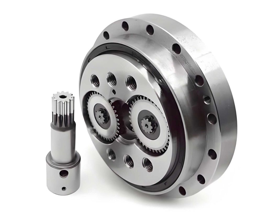
To analyze the transmission behavior under the influence of manufacturing imperfections, a dynamic model is essential. The model developed here simplifies the system for tractability while retaining the critical dynamics. Key assumptions include: treating bearings as rigid bodies, neglecting gravitational forces and tooth friction, assuming ideal axial alignment, using average equivalent stiffness values for similar components, assuming constant input angular velocity, equating deformation displacements between the planetary gear and crankshaft, assuming uniform damping coefficients, and treating the meshing stiffness of both gear stages as time-invariant constants (averaged over an engagement cycle).
The dynamic model for the first-stage (planetary) and second-stage (cycloidal) transmissions can be represented schematically as mass-spring-damper systems. The equations of motion are derived from force and moment balance for each major component: the sun gear, the planetary gear (including its connection to the crankshaft), the cycloidal disc, and the output carrier.
The primary performance metric for a rotary vector reducer is its transmission error, defined as the difference between the ideal output angle (input angle divided by the designed reduction ratio) and the actual measured output angle. This error, denoted as $\Delta \theta$, is the dynamic deviation we aim to control:
$$ \Delta \theta = \frac{\theta_s}{i} – \theta_{ca} $$
where $\theta_s$ is the sun gear (input) angular displacement, $\theta_{ca}$ is the carrier (output) angular displacement, and $i$ is the theoretical reduction ratio.
The dynamic equilibrium equations for the key components are formulated below. The symbols used are defined comprehensively in Table 1.
| Symbol | Description |
|---|---|
| $m_s$, $m_p$, $m_b$, $m_{ca}$ | Mass of sun gear, planetary gear, cycloidal disc, carrier |
| $J_{op}$, $J_{oj}$, $J_o$ | Moment of inertia of planetary gear, cycloidal disc, carrier |
| $x, y$ | Translational displacements |
| $\theta$ | Rotational displacement |
| $F$, $C$ | Meshing force and damping force vectors (with subscripts for component pairs) |
| $R_b$, $R_d$, $R_{dc}$ | Base circle radius, distribution radius of pins, crank radius |
| $e$ | Eccentricity (crank offset) |
| $\omega_c$, $\omega_p$ | Angular velocity of carrier and planetary gear |
| $k$, $c$ | Average meshing stiffness and damping coefficient |
| $\alpha_{jk}$, $\psi_j$, $\phi$ | Engagement angle, phase angle for planet j, assembly phase |
| $T_{out}$ | Output load torque |
Sun Gear:
$$ m_s \ddot{x}_s + F_{sx} + (F + C) \cos A = 0 $$
$$ m_s \ddot{y}_s + F_{sy} + (F + C) \sin A = 0 $$
Planetary Gear:
$$ m_p[\ddot{x}_p – R_{dc}\omega_c^2 \cos(\theta_c + \phi) – R_{dc}\ddot{\theta}_{ca}\sin(\theta_c + \phi) – 2\omega_c \dot{y}_p] – (F + C) \cos A + \sum_{j=1}^{2}(F_{jx} + C_{jx}) + F_{cx} = 0 $$
$$ m_p[\ddot{y}_p – R_{dc}\omega_c^2 \sin(\theta_c + \phi) + R_{dc}\ddot{\theta}_{ca}\cos(\theta_c + \phi) + 2\omega_c \dot{x}_p] – (F + C) \sin A + \sum_{j=1}^{2}(F_{jy} + C_{jy}) + F_{cy} = 0 $$
$$ J_{op}\ddot{\theta}_p – (F + C) R_{bp} – e \sum_{j=1}^{2} [(F_{jix} + C_{jix}) \sin(\theta_p + \psi_j) + (F_{jiy} + C_{jiy}) \cos(\theta_p + \psi_j)] = 0 $$
Cycloidal Disc:
$$ m_b[\ddot{\eta}_{dj}\cos(\theta_p + \psi_j) – e\omega_p^2 \cos(\theta_p + \psi_j) – e\ddot{\theta}_{oj} \sin(\theta_p + \psi_j) – 2\omega_p \dot{\eta}_{dj} \sin(\theta_p + \psi_j)] – (F_{jix} + C_{jix}) + \sum_{k=1}^{m} (F_{ijk} + C_{ijk}) \cos(\alpha_{jk} + \theta_p + \psi_j) = 0 $$
$$ m_b[\ddot{\eta}_{dj} \sin(\theta_p + \psi_j) – e\omega_p^2 \sin(\theta_p + \psi_j) + e\ddot{\theta}_{oj} \cos(\theta_p + \psi_j) + 2\omega_p \dot{\eta}_{dj} \cos(\theta_p + \psi_j)] + (F_{jy} + C_{jy}) + \sum_{k=1}^{m} (F_{jk} + C_{jk}) \sin(\alpha_{jk} + \theta_p + \psi_j) = 0 $$
$$ J_{oj}\ddot{\theta}_{dj} – \sum_{k=1}^{m} (F_{djk} + C_{djk}) R_d \sin \alpha_{jk} – R_{dc}[(F_{jy} + C_{jy}) \cos(\theta_c + \phi_i) – (F_{jx} + C_{jx}) \sin(\theta_c + \phi_i)] = 0 $$
Output Carrier:
$$ m_{ca} \ddot{x}_{ca} – F_{cx} + F_{cax} = 0 $$
$$ m_{ca} \ddot{y}_{ca} – F_{cy} + F_{cay} = 0 $$
$$ J_o \ddot{\theta}_{ca} + F_{cy}R_{dc}\cos(\theta_c + \phi_i) – F_{cix}\sin(\theta_c + \phi_i) = -T_{out} $$
These coupled differential equations can be elegantly expressed in a compact matrix form, which is suitable for numerical simulation and analysis:
$$ \mathbf{M} \ddot{\mathbf{X}} + \mathbf{C} \dot{\mathbf{X}} + \mathbf{K} \mathbf{X} = \mathbf{F} $$
where $\mathbf{M}$, $\mathbf{C}$, and $\mathbf{K}$ are the system mass, damping, and stiffness matrices, respectively; $\mathbf{X}$ is the generalized displacement vector containing all translational and rotational degrees of freedom; and $\mathbf{F}$ is the generalized force vector including input torque, load torque, and excitation forces from errors.
The core objective of performance consistency design is to take a top-level performance requirement—in this case, transmission accuracy—and systematically allocate it to the tolerances of individual design parameters (hard points). The process begins by defining the target performance. For instance, as shown in Table 2, we might aim to improve the transmission error from an initial value of 40 arc-seconds to a target of 20 arc-seconds. A multi-objective genetic optimization algorithm is employed, using the dynamic model as the evaluation function, to find the optimal combination of design parameter nominal values that achieves this target performance.
| Performance Metric | Initial Value (arc-sec) | Target Value (arc-sec) |
|---|---|---|
| Transmission Error ($\Delta \theta$) | 40 | 20 |
Not all design parameters influence the transmission accuracy of the rotary vector reducer equally. Sensitivity analysis is performed to identify parameters with high correlation and coupling to the target performance. This involves perturbing each parameter within the dynamic model and observing the change in the output transmission error. Based on established research and our analysis, the most sensitive parameters for the RV reducer are typically related to the precision of the cycloidal stage and its connection. The key sensitive parameters identified are listed in Table 3 along with their typical functional form of deviation, where $e$ represents a magnitude and the sinusoidal function describes the spatial distribution of the error.
| Sensitive Design Parameter | Deviation Characterization |
|---|---|
| Pin Gear Tooth Profile Deviation | $e \sin(2\theta_k)$ |
| Pin Gear Pitch Cumulative Deviation | $e \sin(2\theta_k)$ |
| Cycloidal Disc Tooth Profile Deviation | $e \sin(2\theta_d)$ |
| Cycloidal Disc Pitch Cumulative Deviation | $e \sin(2\theta_d)$ |
| Crankshaft Eccentric Cam Error | $e$ |
| Bearing Clearance between Cycloidal Disc and Crankshaft | $e$ |
Once the sensitive parameters are identified, the next step is tolerance decomposition. Instead of holding the rigid 20 arc-second target, a permissible tolerance band around this target is defined (e.g., 20 ± 5 arc-seconds). This relaxation at the system level provides the necessary “space” to allocate larger, more economical tolerances to the manufacturing of individual parts. The relationship between the system performance $Y$ (transmission error) and the design parameters $p_i$ can be linearized around their nominal values:
$$ \Delta Y = \sum_{i=1}^{n} S_i \cdot \Delta p_i $$
where $\Delta Y$ is the allowable variation in transmission error (the tolerance band), $S_i$ is the sensitivity coefficient of the $i$-th parameter (obtained from the dynamic model or DOE), and $\Delta p_i$ is the allowable deviation (tolerance) to be allocated to the $i$-th parameter.
This forms a system of linear equations or inequalities. Using methods from interval mathematics and generalized inverse matrices, one can solve for the set of $\Delta p_i$ that satisfies the system-level tolerance $\Delta Y$ while optimizing a secondary objective, such as minimizing total manufacturing cost or maximizing the tolerance zones. The result is a set of optimal tolerance specifications for each key design parameter, as conceptually illustrated in Table 4.
| Design Parameter | Nominal Value | Initial Tight Tolerance | Optimized Relaxed Tolerance |
|---|---|---|---|
| Pin Gear Profile Error Magnitude | 0 µm | ± 2.0 µm | ± 3.5 µm |
| Cycloidal Disc Profile Error Magnitude | 0 µm | ± 1.5 µm | ± 2.8 µm |
| Crankshaft Eccentricity Error | 0 µm | ± 3.0 µm | ± 5.0 µm |
| Bearing Clearance | 0 µm | ± 8.0 µm | ± 12.0 µm |
In conclusion, this research establishes a systematic framework for optimizing the design of rotary vector reducers. By constructing a dynamic model that serves as a high-fidelity bridge between physical design parameters and system-level transmission accuracy, we enable a proactive design-for-manufacturing approach. The methodology involves defining a target performance, identifying parameters with the highest sensitivity through dynamic analysis, and then employing mathematical decomposition techniques to allocate system performance tolerances to individual component tolerances. The key outcome is the ability to specify relaxed, more economically viable tolerance ranges for critical parts like the cycloidal disc, pin gear, and crankshaft, while still guaranteeing the required precision of the final rotary vector reducer assembly. This optimization directly reduces machining difficulty, lowers production costs, and strengthens the competitiveness of the RV reducer in precision drive applications. Future work could involve extending the dynamic model to include more nonlinear effects like time-varying mesh stiffness and friction, and incorporating robust optimization techniques to account for parameter uncertainties.