
The rotary vector reducer, often abbreviated as the RV reducer, is a pivotal component in modern industrial automation, particularly in robotics, due to its exceptional precision, high torque capacity, and compact design. As the demand for industrial robots surges globally, ensuring the quality and reliability of rotary vector reducers becomes increasingly critical. However, the assembly process of these reducers is fraught with challenges, primarily due to the variability in key dimensional parameters of components, which leads to unstable assembly quality. Among the various performance indicators, transmission error stands out as a crucial metric, directly influencing the operational accuracy, noise levels, vibration characteristics, and overall longevity of the reducer. Predicting transmission error prior to assembly can significantly enhance quality control, reduce rework, and optimize part selection, thereby saving time and resources. This article addresses this need by developing a robust prediction model based on a backpropagation (BP) neural network optimized with the sparrow search algorithm (SSA), tailored specifically for rotary vector reducers. The model leverages key component dimensions as inputs to forecast transmission error, offering a practical tool for assembly line decision-making.
In the context of rotary vector reducers, transmission error is defined as the deviation between the actual and theoretical output positions under load, stemming from imperfections in gear meshing and component fits. The reducer typically consists of a two-stage system: a planetary gear stage at the input and a cycloidal pin-wheel stage inside the pin housing. Key components such as the cycloid wheel, crankshaft, pin housing, and planetary gear carrier interact in complex ways, where dimensional tolerances play a significant role. For instance, the span distance of the cycloid wheel, the diameters of eccentric circles on the crankshaft, and the root circle diameter of the pin housing are critical parameters that affect the meshing quality and, consequently, the transmission error. During manufacturing, these parameters often exhibit fluctuations due to machining limitations, especially for high-precision parts like the cycloid wheel. Therefore, identifying and modeling these influences is essential for predictive analytics. The following table summarizes the 15 key parameters selected for this study, which serve as input variables for the prediction model.
| Parameter Symbol | Description |
|---|---|
| x1 | Cycloid wheel span distance (跨棒距) |
| x2 | Diameter of hole 1 in cycloid wheel |
| x3 | Diameter of hole 2 in cycloid wheel |
| x4 | Diameter of eccentric circle 1 on crankshaft |
| x5 | Frictional torque measurement 1 |
| x6 | Diameter of eccentric circle 2 on crankshaft |
| x7 | Frictional torque measurement 2 |
| x8 | Diameter of eccentric circle 3 on crankshaft |
| x9 | Frictional torque measurement 3 |
| x10 | Root circle diameter of pin housing |
| x11 | Inner diameter of hole 1 in planetary carrier |
| x12 | Inner diameter of hole 2 in planetary carrier |
| x13 | Frictional torque of steel balls |
| x14 | Pin diameter |
| x15 | Frictional torque of pins |
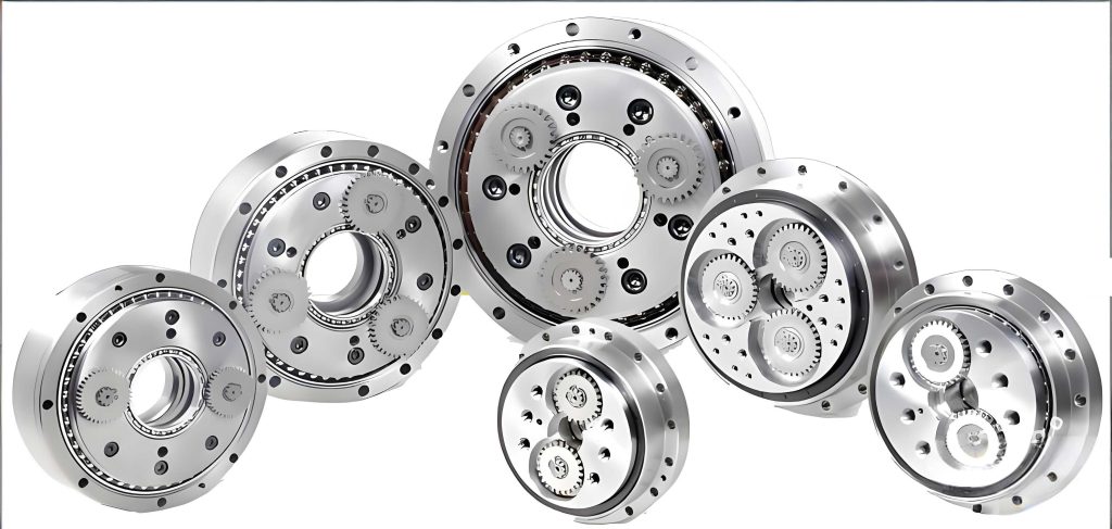
These parameters were chosen based on engineering expertise and prior studies highlighting their impact on the kinematic accuracy of rotary vector reducers. For example, the cycloid wheel span distance (x1) is particularly influential, as it governs the meshing with the pin housing; variations here can lead to significant backlash and transmission error. Similarly, eccentric circle diameters on the crankshaft affect the motion trajectory of the cycloid wheel, while frictional torque measurements indirectly reflect assembly tightness and lubrication conditions. The interplay among these factors is nonlinear, making traditional regression models inadequate. Hence, a neural network approach is adopted to capture these complex relationships. To visualize the structure of a typical rotary vector reducer, the following image provides an illustrative overview.
The backpropagation neural network is a widely used artificial neural network architecture for regression and classification tasks, known for its ability to approximate nonlinear functions. A standard BP network consists of an input layer, one or more hidden layers, and an output layer. Each layer comprises neurons that apply weighted sums and activation functions to transform inputs. For this application, we define the input vector as \(X = [x_1, x_2, \ldots, x_{15}]^T\), representing the 15 key parameters, and the output as \(y\), the transmission error. The hidden layer neurons compute their outputs using a sigmoid activation function, while the output layer uses a linear function. The mathematical formulation is as follows.
Let \(W^{(1)}\) be the weight matrix from the input layer to the hidden layer, with elements \(w_{ji}\) connecting input \(i\) to hidden neuron \(j\), and \(\theta^{(1)}\) be the bias vector for the hidden layer. The net input to hidden neuron \(j\) is:
$$ s_j = \sum_{i=1}^{15} w_{ji} x_i – \theta_j^{(1)} $$
Then, the output of hidden neuron \(j\) is computed using the logistic sigmoid function:
$$ b_j = \frac{1}{1 + \exp(-s_j)} $$
For the output layer, let \(V\) be the weight matrix from the hidden layer to the output layer, with elements \(v_{1j}\) (since only one output neuron is used), and \(\theta^{(2)}\) be the bias for the output neuron. The net input to the output neuron is:
$$ z = \sum_{j=1}^{p} v_{1j} b_j – \theta^{(2)} $$
where \(p\) is the number of hidden neurons. The final output (predicted transmission error) is:
$$ \hat{y} = f(z) $$
with \(f\) being a linear activation function, i.e., \(f(z) = z\). During training, the network minimizes the mean squared error (MSE) between predicted outputs \(\hat{y}\) and actual targets \(y\). The error is propagated backward to adjust weights and biases using gradient descent. The weight update rules for a single iteration are derived from the partial derivatives of the error function. For instance, the update for output layer weights is:
$$ \Delta v_{1j} = \eta \delta b_j $$
where \(\eta\) is the learning rate, and \(\delta\) is the error term for the output neuron, calculated as \(\delta = (y – \hat{y}) \cdot f'(z)\). Similarly, hidden layer weights are updated using error terms propagated from the output layer. This iterative process continues until convergence or a predefined number of epochs. However, BP networks are sensitive to initial weights and can get trapped in local minima, necessitating optimization techniques like the sparrow search algorithm.
The sparrow search algorithm is a novel metaheuristic optimization algorithm inspired by the foraging behavior of sparrows in nature. It simulates sparrows as search agents that explore the solution space, categorized into producers, scroungers, and scouts. Producers actively search for food sources (good solutions), scroungers follow producers, and scouts monitor for predators and danger, enabling escape from local optima. In the context of optimizing a BP network for rotary vector reducer prediction, SSA is used to find the optimal set of weights and biases that minimize the prediction error. The algorithm starts by initializing a population of \(n\) sparrows, each representing a candidate solution vector comprising all weights and biases of the BP network. The fitness of each sparrow is evaluated using the MSE on a training dataset. The position update equations for producers, scroungers, and scouts are as follows.
For a producer (discoverer) sparrow at iteration \(t\), its position \(X_{i,j}^t\) (where \(i\) is the sparrow index and \(j\) is the dimension index) is updated by:
$$ X_{i,j}^{t+1} = \begin{cases} X_{i,j}^t \cdot \exp\left(-\frac{i}{\alpha \cdot T_{\text{max}}}\right) & \text{if } R_2 < ST \\ X_{i,j}^t + Q \cdot L & \text{if } R_2 \geq ST \end{cases} $$
where \(\alpha\) is a random number in \((0,1]\), \(T_{\text{max}}\) is the maximum number of iterations, \(R_2\) is an alarm value in \([0,1]\), \(ST\) is a safety threshold in \([0.5,1]\), \(Q\) is a random number drawn from a normal distribution, and \(L\) is a vector of ones. This equation balances exploration and exploitation based on the alarm level.
For scroungers (followers), the position update is:
$$ X_{i,j}^{t+1} = \begin{cases} Q \cdot \exp\left(\frac{X_{\text{worst}}^t – X_{i,j}^t}{i^2}\right) & \text{if } i > n/2 \\ X_{\text{best}}^{t+1} + |X_{i,j}^t – X_{\text{best}}^{t+1}| \cdot A^+ \cdot L & \text{otherwise} \end{cases} $$
where \(X_{\text{worst}}^t\) and \(X_{\text{best}}^{t+1}\) are the global worst and best positions, respectively, \(A\) is a matrix with random elements of 1 or -1, and \(A^+ = A^T (A A^T)^{-1}\). This allows scroungers to move toward better solutions or explore alternatives.
For scouts (alert sparrows) that sense danger, the position is adjusted by:
$$ X_{i,j}^{t+1} = \begin{cases} X_{\text{best}}^t + \beta \cdot |X_{i,j}^t – X_{\text{best}}^t| & \text{if } f_i > f_g \\ X_{i,j}^t + K \cdot \left( \frac{|X_{i,j}^t – X_{\text{worst}}^t|}{(f_i – f_w) + \epsilon} \right) & \text{if } f_i = f_g \end{cases} $$
where \(\beta\) and \(K\) are step control parameters, \(f_i\) is the fitness of the current sparrow, \(f_g\) and \(f_w\) are the global best and worst fitness values, and \(\epsilon\) is a small constant to avoid division by zero. This mechanism helps escape local optima by diversifying the search. The SSA-BP hybrid approach integrates these updates: initially, the BP network’s weights and biases are encoded into sparrow positions; SSA iteratively optimizes them by evaluating fitness as the MSE on training data; finally, the optimized parameters are decoded back into the BP network for prediction. This synergy enhances the global search capability and convergence speed, making it suitable for complex problems like transmission error prediction in rotary vector reducers.
To validate the SSA-BP model, an empirical study was conducted using data collected from the assembly line of a 42N-126 type rotary vector reducer. A total of 114 samples were obtained, each comprising measurements of the 15 input parameters and the corresponding transmission error value. The dataset was split into 89 samples for training and 25 samples for testing, ensuring a representative distribution. Prior to model training, data preprocessing was performed to remove outliers and normalize the features to a [-1, 1] range, which accelerates convergence and mitigates scaling issues. The normalization formula applied to each parameter \(x\) is:
$$ x^* = (y_{\text{max}} – y_{\text{min}}) \frac{x – x_{\text{min}}}{x_{\text{max}} – x_{\text{min}}} + y_{\text{min}} $$
where \(x_{\text{max}}\) and \(x_{\text{min}}\) are the maximum and minimum values of the parameter in the dataset, and \(y_{\text{max}} = 1\), \(y_{\text{min}} = -1\). A subset of the normalized data is shown in the table below to illustrate the preprocessing outcome.
| Sample | x1 | x2 | x3 | x4 | x5 | … | Transmission Error (y) |
|---|---|---|---|---|---|---|---|
| 1 | -0.7575 | -0.5682 | 0.2000 | 0.9831 | -1.0000 | … | -0.0833 |
| 2 | -0.8623 | -0.7045 | -0.6941 | 0.9812 | 0.6000 | … | 0.4167 |
| 3 | -0.7827 | -0.2422 | 0.4353 | 0.9673 | -0.2000 | … | 0.5833 |
| 4 | -0.8021 | -0.3864 | 0.2706 | 0.9871 | -0.6000 | … | 0.1677 |
| 5 | -0.7905 | -0.5227 | 0.1294 | 0.9841 | -1.0000 | … | 0.0000 |
The BP network architecture was configured with 15 input neurons (matching the parameters), 10 hidden neurons (determined empirically using the rule \(l = \sqrt{m + n} + a\), where \(m=15\), \(n=1\), and \(a\) is a constant between 1 and 10), and 1 output neuron for transmission error. The hidden layer activation function was set to logistic sigmoid, the output layer to linear, and the training algorithm to Levenberg-Marquardt (trainlm) with a learning rate of 0.01. The performance goal was set to 10-5 MSE. For SSA optimization, the population size was 20 sparrows, maximum iterations 20, search bounds for weights and biases set to [-5, 5], alarm value \(R_2 = 0.6\), producer proportion 0.7, and scout proportion 0.2. The fitness function for SSA was defined as the combined MSE of training and testing sets:
$$ f = \text{argmin} \left( \text{mse}_{\text{train}} + \text{mse}_{\text{test}} \right) $$
where mse denotes mean squared error. This encourages the algorithm to find solutions that generalize well. The optimization process was implemented in MATLAB R2012b, with the SSA iteratively tuning the BP network’s initial weights and biases before training.
The results demonstrate the efficacy of the SSA-BP model for predicting transmission error in rotary vector reducers. Compared to a standard BP network without optimization, the SSA-BP model showed superior prediction accuracy and stability. The prediction curves for both models on the test dataset are illustrated conceptually: the SSA-BP predictions closely align with the actual transmission error values, while the BP predictions exhibit larger deviations. This is quantified by the mean squared error metrics, as summarized in the table below.
| Model | Mean Squared Error (MSE) |
|---|---|
| Standard BP Neural Network | 0.025146 |
| SSA-Optimized BP Neural Network | 0.0088254 |
The SSA-BP model achieved an MSE of 0.0088254, which is approximately 65% lower than that of the standard BP model (0.025146), indicating a significant improvement in prediction precision. This reduction in error translates to more reliable forecasts of transmission error, enabling better part selection during assembly of rotary vector reducers. Additionally, the convergence curve of the SSA-BP model during training showed a steady decline in error over iterations, confirming the algorithm’s ability to escape local minima and approach a global optimum. The error distribution for the SSA-BP model was also more concentrated around zero compared to the broader spread observed in the BP model, further validating its robustness. These findings underscore the value of integrating metaheuristic optimization with neural networks for complex industrial applications like rotary vector reducer quality prediction.
In conclusion, this study presents a novel approach to predicting transmission error in rotary vector reducers using a sparrow search algorithm-optimized backpropagation neural network. By leveraging key dimensional parameters of components as inputs, the model effectively captures the nonlinear relationships influencing assembly quality. The SSA optimization enhances the BP network’s performance by optimizing initial weights and biases, leading to higher accuracy and stability in predictions. The empirical results from a 42N-126 type rotary vector reducer dataset confirm that the SSA-BP model outperforms a standard BP model, with a substantially lower mean squared error. This predictive tool can assist manufacturers in pre-assembly part selection, reducing rework rates, minimizing resource waste, and improving overall product quality for rotary vector reducers. Future work may explore additional influencing factors such as environmental conditions or human operator variables, as well as other advanced optimization algorithms, to further refine the prediction model for rotary vector reducers in diverse industrial settings.