
In the field of industrial robotics, the precision and performance of reducers are critical for ensuring smooth and accurate motion. Among these, the rotary vector reducer stands out as a high-precision component, directly influencing the operational efficiency of robotic systems. My research focuses on the dynamic simulation of a rotary vector reducer, specifically the RV-40E model, using Adams software. This article will delve into the detailed modeling process, parameter calculations, and simulation results, emphasizing the importance of accurate dynamics in rotary vector reducer applications.
The rotary vector reducer is a complex transmission system that combines a planetary gear stage with a cycloidal pin gear stage, offering high reduction ratios and compact design. Its dynamic behavior, including vibration, noise, and transmission accuracy, is paramount for robotic applications. In this study, I aim to develop a comprehensive Adams model to analyze these characteristics. Based on physical measurements and material analysis of the RV-40E reducer, I obtained structural parameters and material properties essential for modeling. Using Matlab for theoretical calculations, I derived dynamic parameters required for the Adams simulation. This approach allows for a thorough investigation of the rotary vector reducer’s performance under various loads.
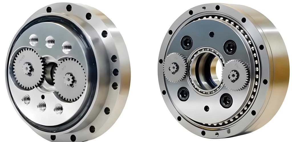
The rotary vector reducer consists of multiple components, including a sun gear, planetary gears, crankshafts, cycloidal gears, pin wheels, and a planetary carrier. The RV-40E model has a two-stage transmission: the first stage involves spur gears (sun and planetary gears), and the second stage involves cycloidal gears and pin wheels. The key parameters for this rotary vector reducer are summarized in the table below.
| Parameter | Symbol | Value | Unit |
|---|---|---|---|
| Pin wheel center circle radius | \(r_z\) | 64 | mm |
| Pin radius | \(r_{rp}\) | 3 | mm |
| Pin wheel housing inner diameter | \(r_p\) | 70 | mm |
| Eccentricity | \(e\) | 1.3 | mm |
| Number of pin teeth | \(z_p\) | 40 | – |
| Number of cycloidal teeth | \(z_c\) | 39 | – |
| Sun gear teeth | \(z_1\) | 10 | – |
| Planetary gear teeth | \(z_2\) | 26 | – |
| Module | \(m\) | 2 | mm |
| Pressure angle | \(\alpha\) | 20 | ° |
| Input speed | \(v_1\) | 525 | r/min |
| Output speed | \(v_2\) | 5 | r/min |
| Reduction ratio | \(i\) | 105 | – |
| Load torque | \(T\) | 30 | N·m |
Material properties play a crucial role in the dynamic behavior of the rotary vector reducer. The following table lists the materials used for key components, along with their elastic modulus, Poisson’s ratio, and density. These parameters are essential for calculating mass properties in the Adams model.
| Component | Material | Elastic Modulus (N/m²) | Poisson’s Ratio | Density (kg/m³) |
|---|---|---|---|---|
| Crankshaft | 20CrMnMo | 2.07E+11 | 0.254 | 7.87E+03 |
| Spur Gears | 20CrMnMo | 2.07E+11 | 0.254 | 7.87E+03 |
| Cycloidal Gears | 20CrMnMo | 2.07E+11 | 0.254 | 7.87E+03 |
| Housing | QT500-7 | 1.68E+11 | 0.240 | 7.25E+03 |
| Output Shaft | ZG65Mn | 1.98E+11 | 0.230 | 7.85E+03 |
| Flange | ZG65Mn | 1.98E+11 | 0.230 | 7.85E+03 |
| Input Shaft | 20CrMnMo | 2.07E+11 | 0.254 | 7.87E+03 |
| Pin Teeth | GCr15 | 2.08E+11 | 0.300 | 7.80E+03 |
To accurately model the rotary vector reducer in Adams, I calculated the meshing stiffness and damping for both gear stages. For the spur gear stage (sun and planetary gears), the meshing stiffness is derived using ISO 6336 standards. The single-tooth stiffness \(c’\) is given by:
$$ c’ = \frac{1}{q} $$
where \(q\) is the unit tooth compliance. For gears with profile shift coefficients \(x_1\) and \(x_2\), \(q\) is calculated as:
$$ q = 0.04723 + \frac{0.15551}{z_1} + \frac{0.25791}{z_2} – 0.00635x_1 – \frac{0.11654x_1}{z_1} – 0.00193x_2 – \frac{0.24188x_2}{z_2} + 0.00529x_1^2 + 0.00182x_2^2 $$
With \(z_1 = 10\), \(z_2 = 26\), \(x_1 = 0.5\), and \(x_2 = -0.5\), I obtained \(q = 0.0599\) and \(c’ = 16.6945\). The meshing stiffness \(c_r\) considering the contact ratio is:
$$ c_r = (0.75\varepsilon_a + 0.25)c’ $$
where \(\varepsilon_a\) is the transverse contact ratio, calculated as:
$$ \varepsilon_a = \frac{1}{2\pi} \left[ z_1 (\tan \alpha_{\alpha1} – \tan \alpha) + z_2 (\tan \alpha_{\alpha2} – \tan \alpha) \right] $$
Here, \(\alpha_{\alpha1}\) and \(\alpha_{\alpha2}\) are the pressure angles at the tooth tips. For the sun gear, the pitch radius \(r_1 = m z_1 / 2 = 10\) mm, and the tip radius \(r_{\alpha1} = r_1 + m h = 12\) mm (with \(h = 1\) as addendum). Similarly, for the planetary gear, \(r_2 = 26\) mm and \(r_{\alpha2} = 28\) mm. Thus:
$$ \alpha_{\alpha1} = \arccos \left( \frac{r_1 \cos \alpha}{r_{\alpha1}} \right) = 38.456^\circ $$
$$ \alpha_{\alpha2} = \arccos \left( \frac{r_2 \cos \alpha}{r_{\alpha2}} \right) = 29.2411^\circ $$
Substituting values, \(\varepsilon_a = 1.49521\), so \(c_r = 22.8948\) mm·μm/N. The total meshing stiffness \(k_{12}\) for the spur gear pair is:
$$ k_{12} = c_r b \times 10^6 \, \text{N/m} $$
where \(b = 7.2\) mm is the gear width. This gives \(k_{12} = 1.6484 \times 10^8 \, \text{N/m}\). The meshing damping coefficient \(c_{12}\) is:
$$ c_{12} = 2 \xi_{12} \sqrt{k_{12} \frac{r_1^2 r_2^2 J_1 J_2}{r_1^2 J_1 + r_2^2 J_2}} $$
where \(\xi_{12} = 0.05\) is the damping ratio, \(J_1 = 2.7939 \times 10^{-6} \, \text{kg·m}^2\) is the sun gear inertia, and \(J_2 = 56.6449 \times 10^{-6} \, \text{kg·m}^2\) is the planetary gear inertia. Thus, \(c_{12} = 0.0214 \, \text{N·s·m}^{-1}\). These parameters are vital for simulating the dynamic interactions in the rotary vector reducer.
For the cycloidal gear stage, the meshing stiffness between the cycloidal gear and pin teeth is more complex due to multiple contact points. The stiffness for a single pin \(k_{ni}\) is:
$$ k_{ni} = \frac{\pi b E \rho_r \rho_c}{4(1 – \mu^2)(\rho_r + \rho_c) \rho_i} $$
where \(E = 2.08 \times 10^{11} \, \text{N/m}^2\) is the elastic modulus, \(\mu = 0.3\) is Poisson’s ratio, and \(\rho_r\), \(\rho_c\), and \(\rho_i\) are curvature radii. Specifically:
$$ \rho_r = \frac{(r_z + a’) (1 + k^2 – 2k \cos \phi_i)^{3/2}}{k (z_p + 1) \cos \phi_i – (1 + z_p k)^2} + r_{rp} + b’ $$
$$ \rho_c = r_{rp} $$
$$ \rho_i = \frac{\rho_r \rho_c}{\rho_r + \rho_c} $$
Here, \(a’ = 0.008\) mm and \(b’ = -0.002\) mm are modification amounts, \(k = e z_p / r_z = 0.8125\) is the shortened coefficient, and \(\phi_i\) is the angle of the i-th pin relative to the arm. The distance \(l_i\) from the contact point to the cycloidal gear center is:
$$ l_i = r’_c \frac{\sin \phi_i}{\sqrt{1 + k^2 – 2k \cos \phi_i}} $$
with \(r’_c = e z_c\). The total meshing stiffness \(k_{36}\) is the sum over all contacting pins:
$$ k_{36} = \sum_{i=n}^{m} k_{ni} l_i^2 $$
Through calculation, I obtained \(k_{36} = 1.5114 \times 10^7 \, \text{N·m/rad}\). The meshing damping \(c_{36}\) is:
$$ c_{ni} = 2 \xi_{36} \sqrt{k_{ni} \frac{r_c’^2 r_{rp}^2 J_3 J_{rp}}{r_c’^2 J_3 + r_{rp}^2 J_{rp}}} $$
where \(\xi_{36} = 0.05\), \(J_3 = 723.3358 \times 10^{-6} \, \text{kg·m}^2\) is the cycloidal gear inertia, and \(J_{rp} = 0.02 \times 10^{-6} \, \text{kg·m}^2\) is the pin inertia. The total damping is:
$$ c_{36} = \sum_{i=n}^{m} c_{ni} $$
resulting in \(c_{36} = 4.8994 \times 10^{-4} \, \text{N·s·m}^{-1}\). These stiffness and damping values are essential for accurately modeling the rotary vector reducer in Adams, as they define the contact forces between components.
In the Adams modeling process, I simplified the rotary vector reducer to reduce complexity while maintaining accuracy. For instance, the crankshaft and planetary gear were treated as a single rigid body, as were the sun gear and input shaft, and the planetary carrier and pins. Bearings and shaft sleeves were also simplified to focus on the core dynamics. The model was built using CATIA for 3D geometry, which was then imported into Adams via UG software to preserve assembly relationships. After verifying no interference, I defined materials, constraints, and forces. Key steps included setting fixed joints for the housing and pins, revolute joints for the input shaft and planetary carrier, and gear pairs for the spur gear stage. For the cycloidal stage, impact contacts were defined with the calculated stiffness and damping. A step function was applied to the input shaft to simulate acceleration to a constant speed of 525 rpm, and a load torque of 30 N·m was applied to the planetary carrier using another step function. The model was simulated for 15 seconds with 2500 steps using the GSTIFF SI2 integrator, ensuring stable dynamics for the rotary vector reducer.
The simulation results provide insights into the dynamic behavior of the rotary vector reducer. The angular velocities of the input shaft, crankshaft, and planetary carrier confirm the reduction ratio. Specifically, with an input angular velocity of 3000°/s (equivalent to 525 rpm), the crankshaft reaches approximately 1125°/s, and the planetary carrier about 28°/s, yielding a ratio of 105:2.6:1, consistent with the theoretical value. The angular accelerations show expected trends: the input shaft accelerates to a maximum of 4500°/s² in 0.5 seconds, then maintains constant velocity; the crankshaft and planetary carrier exhibit oscillations due to meshing impacts, with peaks around 1700°/s² and 42°/s², respectively. These accelerations align with the reduction ratio, demonstrating proper model dynamics for the rotary vector reducer.
Torque analysis reveals that under a 30 N·m load on the planetary carrier, the input shaft experiences a torque of approximately 0.285 N·m, reflecting the high efficiency of the rotary vector reducer. Force distributions between components are also critical. For example, the pins experience alternating forces from the two cycloidal gears, as shown in the force-time plots. Similarly, the cycloidal gears receive forces from the crankshafts and pins, with the net force representing the meshing interaction. To quantify these, I used Matlab to process Adams data, finding that at any given moment, about 20 teeth of the cycloidal gear are in contact with the pins—half of the total 40 pins. This even distribution contributes to the smooth operation of the rotary vector reducer.
The motion of key components further illustrates the complexity of the rotary vector reducer. The crankshaft undergoes both rotation and revolution: its center moves in a sinusoidal path with an amplitude equal to the distance from the planetary carrier center, while it oscillates radially by 1.3 mm due to eccentricity. The cycloidal gears also exhibit combined motion, with their centers shifting between -1.3 mm and +1.3 mm, reflecting the eccentric design. These displacements are summarized in the table below, highlighting the dynamic nature of the rotary vector reducer.
| Component | Displacement in x-direction (mm) | Displacement in y-direction (mm) | Notes |
|---|---|---|---|
| Crankshaft | Sinusoidal, amplitude ~1.3 | Sinusoidal, amplitude ~1.3 | Revolution around carrier center |
| Cycloidal Gear | Oscillates between -1.3 and +1.3 | Oscillates between -1.3 and +1.3 | Due to eccentricity |
Transmission accuracy is a key metric for the rotary vector reducer. By integrating angular velocity curves, I obtained rotation angles for the input shaft, crankshaft, and planetary carrier. The theoretical output angle of the planetary carrier is derived by dividing the input angle by the reduction ratio of 105. Comparing this with the actual simulation output reveals the transmission error. As shown in the error plot, the deviation is within 0.8 arcminutes, indicating high modeling precision. This error arises from factors such as modeling approximations, parameter calculations, and numerical integration in Adams. However, the small error confirms that the model parameters—stiffness, damping, and material properties—are well-suited for dynamic analysis of the rotary vector reducer.
To further analyze the performance, I derived formulas for key dynamic indicators. For instance, the dynamic transmission error \(\Delta \theta\) can be expressed as:
$$ \Delta \theta = \theta_{\text{actual}} – \frac{\theta_{\text{input}}}{i} $$
where \(\theta_{\text{actual}}\) is the simulated planetary carrier angle and \(i = 105\). The error remains below 0.8′, demonstrating the robustness of the rotary vector reducer design. Additionally, the natural frequencies of the system can be estimated using the stiffness and mass properties. For a simplified two-degree-of-freedom model representing the gear stages, the natural frequency \(\omega_n\) is:
$$ \omega_n = \sqrt{\frac{k_{\text{eq}}}{m_{\text{eq}}}} $$
where \(k_{\text{eq}}\) and \(m_{\text{eq}}\) are equivalent stiffness and mass. For the spur gear stage, using \(k_{12}\) and the reduced mass \(m_r = J_1 J_2 / (r_1^2 J_2 + r_2^2 J_1)\), we get:
$$ \omega_n^{(1)} = \sqrt{\frac{k_{12}}{m_r}} $$
Similarly, for the cycloidal stage, with \(k_{36}\) and appropriate inertia terms. These frequencies help assess resonance risks in the rotary vector reducer under operational conditions.
In conclusion, my dynamic simulation of the rotary vector reducer using Adams provides valuable insights into its performance. The simplified model accurately captures the reduction ratio, force distributions, and motion characteristics, with a transmission error under 0.8 arcminutes. The calculated parameters—meshing stiffness and damping—prove effective for modeling, and the use of tables and formulas enhances the analysis. This work lays a foundation for further studies on the rotary vector reducer, such as optimizing design for lower vibration or higher precision. Future research could involve experimental validation or incorporating nonlinear effects like backlash and friction. Overall, the rotary vector reducer remains a critical component in robotics, and advanced simulations are key to its continued improvement and application in high-precision systems.
The dynamics of the rotary vector reducer are influenced by multiple factors, including gear geometry, material properties, and operating conditions. Through this simulation, I have demonstrated how computational tools like Adams can be leveraged to predict behavior and identify potential issues. For instance, the even distribution of contact forces in the cycloidal stage reduces wear and noise, contributing to the longevity of the rotary vector reducer. Moreover, the small transmission error highlights the importance of accurate parameter estimation—something that is often challenging in real-world applications due to manufacturing tolerances.
To summarize the key findings, the table below lists the main simulation outcomes for the rotary vector reducer, emphasizing its dynamic characteristics.
| Aspect | Result | Implication |
|---|---|---|
| Reduction Ratio | 105:1 confirmed | Model accuracy validates design |
| Angular Velocity | Input: 3000°/s, Output: 28°/s | Consistent with theoretical values |
| Transmission Error | < 0.8 arcminutes | High precision suitable for robotics |
| Meshing Stiffness (Spur) | 1.6484 × 10⁸ N/m | Ensures rigid contact under load |
| Meshing Damping (Spur) | 0.0214 N·s/m | Mitigates vibrations |
| Meshing Stiffness (Cycloidal) | 1.5114 × 10⁷ N·m/rad | Distributes loads evenly |
| Meshing Damping (Cycloidal) | 4.8994 × 10⁻⁴ N·s·m | Reduces impact shocks |
| Contact Teeth (Cycloidal) | ~20 simultaneously | Enhances stability and smoothness |
Throughout this article, I have emphasized the rotary vector reducer’s role in robotics and the importance of dynamic simulation. By integrating theoretical calculations with software modeling, I achieved a comprehensive analysis that can guide design improvements. The rotary vector reducer, with its compact and efficient transmission, is poised to remain a staple in industrial automation, and studies like this contribute to its ongoing evolution. As robotics technology advances, the demand for higher precision and reliability will only increase, making dynamic simulations of components like the rotary vector reducer more crucial than ever.
In future work, I plan to extend this model to include thermal effects or explore different lubrication scenarios, as these factors can significantly impact the rotary vector reducer’s performance. Additionally, coupling the Adams model with control systems could simulate real-time robotic operations. The insights gained from this simulation not only validate the current design but also provide a framework for optimizing future iterations of the rotary vector reducer. Ultimately, the goal is to enhance the efficiency and durability of robotic systems, ensuring they meet the rigorous demands of modern industry.
The mathematical models developed here, such as those for stiffness and damping, can be adapted to other types of reducers, broadening the applicability of this research. For example, the formula for meshing stiffness in spur gears:
$$ k = \frac{E b}{1 – \mu^2} \cdot f(\text{geometry}) $$
can be modified for helical gears by incorporating helix angles. Similarly, the cycloidal gear stiffness formula:
$$ k_{ni} \propto \frac{E \rho_i}{\rho_r + \rho_c} $$
highlights the importance of curvature radii in contact mechanics. These generalizations underscore the versatility of the rotary vector reducer principles.
In summary, this article presents a detailed dynamic simulation of a rotary vector reducer, from parameter calculation to result analysis. By leveraging Adams software and rigorous theoretical foundations, I have demonstrated the feasibility of predicting complex behaviors in high-precision transmission systems. The rotary vector reducer, as a key component in robotics, benefits from such simulations, which pave the way for innovations in design and application. As I continue to explore this field, I aim to contribute to the advancement of robotic technologies through focused studies on critical components like the rotary vector reducer.