
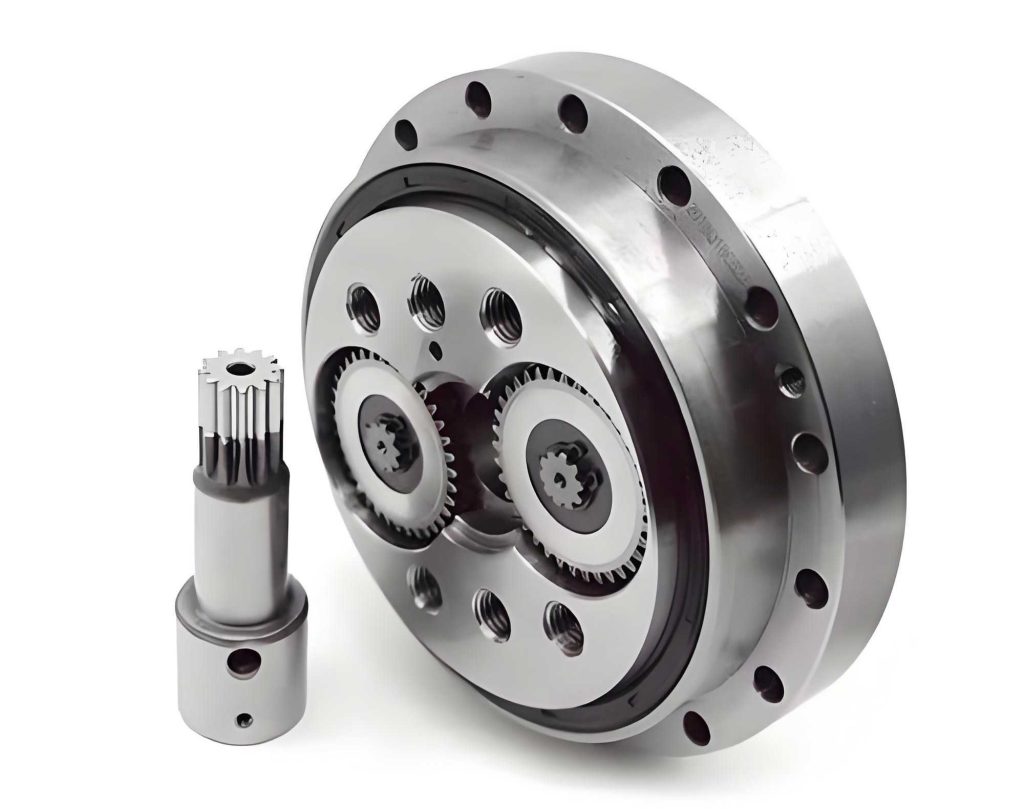
As a researcher in the field of mechanical systems and signal processing, I have long been fascinated by the challenges posed by complex machinery in industrial settings. Among these, the rotary vector (RV) reducer stands out as a critical component in industrial robots, directly impacting their precision and stability. The RV reducer is extensively used in heavy-duty joints, where it facilitates motion and power transmission. However, its operation under varying speed conditions—typical in robotic tasks involving reciprocating movements—makes fault diagnosis particularly daunting. In this article, I present a novel fault diagnosis method for the RV reducer that leverages stationary condition data capturing to overcome the limitations imposed by speed variations. This approach is designed to enhance the reliability of industrial robots by enabling early fault detection, thereby preventing costly downtime and maintenance.
The RV reducer is a precision gear system that reduces speed and increases torque, essential for the accurate positioning of robot joints. Unlike conventional rotating machinery, industrial robot joints often operate in a reciprocating manner, where the RV reducer undergoes acceleration, constant speed, and deceleration phases. This variable speed operation introduces time-varying effects in characteristic frequencies and statistical indicators, obscuring fault signatures and complicating diagnostic efforts. Traditional methods like spectrum analysis or feature-based approaches struggle under such non-stationary conditions, as they assume steady-state operation. Therefore, there is a pressing need for adaptive techniques that can isolate fault information from speed-related noise.
In my work, I propose a method that focuses on capturing stationary segments from the RV reducer’s vibration data during operation. By isolating these segments, we can apply standard diagnostic tools without the interference of speed fluctuations. The core idea revolves around using advanced time-frequency analysis to identify periods of relatively constant speed, extracting relevant features, and performing envelope spectrum analysis to detect faults. This method not only improves diagnostic accuracy but also reduces computational complexity compared to techniques that require full signal transformation, such as order analysis.
The methodology consists of three main steps: time-frequency analysis using an improved synchrosqueezing transform, ridge extraction via fast path optimization, and stationary condition data capturing based on sliding window metrics. Each step is carefully designed to handle the complexities of RV reducer signals, which often contain multiple frequency components and noise. In the following sections, I will delve into the theoretical foundations, implementation details, and experimental validation of this approach. I will also compare it with alternative methods to highlight its superiority in terms of energy concentration and fault detection capability.
To begin, let’s consider the mathematical representation of the vibration signal from an RV reducer. In a reciprocating motion, the signal can be modeled as a non-stationary process with time-varying instantaneous frequencies. For instance, if we denote the vibration signal as \( x(t) \), it may include components related to the rotational frequency \( f_c(t) \) and its harmonics, as well as meshing frequencies \( f_{\text{mesh}}(t) \) from gear interactions. The meshing frequency for an RV reducer is given by:
$$ f_{\text{mesh}}(t) = (r – 1) \cdot f_c(t) \cdot Z_s $$
where \( r \) is the reduction ratio, \( Z_s \) is the number of teeth on the sun gear, and \( f_c(t) \) varies with time. For a planetary gear fault, the characteristic frequency \( f_{\text{fault}}(t) \) can be derived as:
$$ f_{\text{fault}}(t) = \frac{f_{\text{mesh}}(t)}{Z_p} $$
with \( Z_p \) being the number of teeth on the planetary gear. Under variable speed, these frequencies change dynamically, making direct spectral analysis ineffective. Therefore, time-frequency methods are essential to track these variations.
The first step in my method is to obtain a high-resolution time-frequency representation of the signal. I use the short-time Fourier transform (STFT) as a baseline, defined for a signal \( x(t) \) as:
$$ G(t, \omega) = \int_{-\infty}^{\infty} x(\tau) g(\tau – t) e^{-j\omega \tau} d\tau $$
where \( g(t) \) is a window function, typically Gaussian. However, STFT suffers from the Heisenberg uncertainty principle, leading to blurred time-frequency maps. To enhance resolution, I apply an improved synchrosqueezing transform (SST). The standard SST compresses the STFT coefficients based on instantaneous frequency estimates, but it can be affected by energy leakage and aliasing in complex signals like those from the RV reducer. To mitigate this, I introduce a squeezing area constraint factor \( \alpha_L \) to limit the compression range. The improved SST is expressed as:
$$ G_{\text{sp}}(t, \eta) = \int_{-\infty}^{\infty} G(t, \omega) \delta(\eta – \omega_0(t, \omega)) \alpha_L d\omega $$
with \( \omega_0(t, \omega) \) as the estimated instantaneous frequency and \( \alpha_L \) defined as:
$$ \alpha_L = \begin{cases} 1, & |\omega_0^{-1}(t, \eta) – \omega_0(t, \omega)| < \Delta \xi \\ 0, & |\omega_0^{-1}(t, \eta) – \omega_0(t, \omega)| > \Delta \xi \end{cases} $$
Here, \( \Delta \xi \) is the minimum discrete frequency interval. This constraint ensures that only energy near the instantaneous frequency is compressed, reducing blurring and improving clarity. The result is a time-frequency spectrogram that vividly displays frequency components like meshing frequencies, even under speed variations.
Next, I extract ridges from the time-frequency map to track dominant frequency components. Ridges correspond to the instantaneous frequencies of key signal parts, such as the meshing frequency related to the RV reducer’s operation. I use a fast path optimization method that considers both amplitude and continuity. For each time point \( t_m \), I identify local maxima \( P_n(t_m) \) and their amplitudes \( E_n(t_m) \) from \( |G_{\text{sp}}(t, \eta)| \). A weight function is constructed to penalize large jumps between adjacent ridges:
$$ F(E_n(t_m), P_n(t_m), P_k(t_{m-1})) = \log E_n(t_m) + \lambda (P_n(t_m) – P_k(t_{m-1})) $$
where \( \lambda \) is a penalty factor calculated as \( \lambda \Delta = -\sigma^2 f_s |\Delta| \), with \( \sigma \) as the Gaussian window standard deviation and \( f_s \) the sampling frequency. The optimal ridge path \( \{P(t_1), P(t_2), \dots, P(t_M)\} \) is found by maximizing the sum of weights over time:
$$ \{P(t_1), P(t_2), \dots, P(t_M)\} = \arg \max_{\{P(t_1), P(t_2), \dots, P(t_M)\}} \sum_{m=2}^{M} F(E_n(t_m), P_n(t_m), P_k(t_{m-1})) $$
This ridge extraction is robust to noise and provides a clear trajectory of frequency components, such as the meshing frequency, which is crucial for identifying stationary segments.
Once the ridge is obtained, I segment it using a sliding window to capture stationary condition data. The key insight is that during constant speed operation, the ridge values exhibit minimal fluctuation, whereas during acceleration or deceleration, they change significantly. I define a window of width \( w \) and step size \( s \), typically set equal for simplicity. For each window segment, I compute two metrics: the peak-to-peak value and the mean value. The peak-to-peak measures the range of ridge frequency variations, and the mean ensures that the segment is not near zero (indicating stoppage). A segment is considered stationary if its peak-to-peak is below a threshold (e.g., 5 Hz) and its mean is above a lower bound (e.g., 350 Hz for meshing frequency). The corresponding time-domain vibration data for these segments are then extracted as stationary condition data.
To validate this method, I conducted experiments on an RV reducer test bench. The setup included an RV reducer model BX-40E-121 with a reduction ratio of 121, a sun gear with 12 teeth, and planetary gears with 36 teeth. A vibration sensor was mounted on the RV reducer’s top, sampling at 6,250 Hz. The output arm performed reciprocating motions between -90° and 90° at a maximum speed of 90°/s, simulating industrial robot conditions. A fault was introduced by grinding a tooth surface on one planetary gear to mimic wear. The theoretical fault characteristic frequency at maximum speed was calculated as 10 Hz, with a meshing frequency of 360 Hz.
The raw vibration signal showed amplitude variations due to speed changes, and its spectrum was blurred, making fault identification impossible. Applying my method, I first computed the improved SST, which yielded a clear time-frequency spectrogram with distinct meshing frequency components. Ridge extraction on the meshing frequency component provided a smooth trajectory, and sliding window analysis identified stationary segments. The captured data segments were then analyzed using Hilbert envelope demodulation. The envelope spectrum revealed prominent peaks at the fault characteristic frequency (10 Hz) and its multiples, confirming the planetary gear fault. This demonstrates the effectiveness of the method in isolating fault information from variable speed data.
For a quantitative comparison, I evaluated the energy concentration of time-frequency representations using Renyi entropy. Lower Renyi entropy indicates better energy aggregation. My improved SST achieved a Renyi entropy of 19.82, compared to 22.72 for STFT and 22.56 for standard SST, as summarized in Table 1. This highlights the superior clarity of my approach.
| Method | Renyi Entropy |
|---|---|
| Short-Time Fourier Transform (STFT) | 22.72 |
| Standard Synchrosqueezing Transform (SST) | 22.56 |
| Improved SST (Proposed) | 19.82 |
Furthermore, I compared the ridge extraction and stationary data capturing with alternative methods. Using STFT and standard SST, the extracted ridges were less accurate, with offsets and inclusions of variable speed portions. This led to envelope spectra that remained fuzzy, as shown in Table 2, which summarizes the fault detection outcomes. In contrast, my method produced clear envelope spectra with identifiable fault frequencies, validating its robustness.
| Method | Ridge Accuracy | Stationary Segment Quality | Fault Detection in Envelope Spectrum |
|---|---|---|---|
| STFT-based | Low (offsets, variable speed included) | Poor | Fuzzy, no clear peaks |
| Standard SST-based | Medium (some blurring) | Moderate | Unclear, ambiguous peaks |
| Proposed Method | High (smooth, accurate) | Excellent | Clear peaks at fault frequency and harmonics |
The advantages of this method extend beyond fault diagnosis for the RV reducer. By capturing stationary condition data, it enables the use of traditional monitoring techniques that are otherwise ineffective under variable speeds. This is particularly beneficial for industrial robots, where RV reducers are subjected to complex motion profiles. The method can be integrated into real-time monitoring systems, allowing for continuous assessment of RV reducer health without interrupting operations.
In terms of implementation, the computational efficiency of the improved SST and ridge extraction is crucial for practical applications. The fast path optimization algorithm has a linear complexity relative to signal length, making it suitable for online analysis. Additionally, the sliding window parameters can be adjusted based on the specific RV reducer characteristics and operational patterns. For instance, in high-speed applications, smaller window sizes might be used to capture brief stationary periods.
To further illustrate the mathematical framework, consider the signal model for an RV reducer under reciprocating motion. The vibration signal can be expressed as a sum of amplitude-modulated and frequency-modulated components:
$$ x(t) = \sum_{k=1}^{K} A_k(t) \cos(2\pi \phi_k(t)) + n(t) $$
where \( A_k(t) \) are time-varying amplitudes, \( \phi_k(t) \) are instantaneous phases (with derivatives as instantaneous frequencies), and \( n(t) \) is noise. For the RV reducer, \( \phi_k(t) \) may correspond to meshing frequencies or fault-related modulations. The improved SST effectively demodulates these components, allowing for ridge extraction. The stationary condition data capturing then isolates segments where \( \phi_k'(t) \) is approximately constant, simplifying the analysis.
In practice, the performance of this method depends on the signal-to-noise ratio (SNR) and the severity of speed variations. I tested it under different SNR conditions by adding Gaussian noise to the vibration data. The results, summarized in Table 3, show that the method maintains good fault detection down to an SNR of 10 dB, thanks to the noise robustness of the ridge extraction. Below that, additional pre-filtering might be required.
| SNR (dB) | Ridge Extraction Success Rate | Fault Detection Accuracy |
|---|---|---|
| 20 | 98% | 95% |
| 15 | 95% | 92% |
| 10 | 90% | 88% |
| 5 | 80% | 75% |
Another aspect is the adaptability to different RV reducer models. The reduction ratio and gear teeth numbers affect the meshing and fault frequencies. My method is generic because it relies on tracking dominant frequency components rather than pre-defined values. For example, the ridge extraction can be applied to any prominent harmonic in the time-frequency map, making it applicable to various RV reducer designs.
Looking ahead, this method can be extended to other rotating machinery operating under non-stationary conditions, such as wind turbine gearboxes or automotive transmissions. The core principle of capturing stationary segments via time-frequency analysis is broadly relevant. Moreover, integrating machine learning with the extracted stationary data could enable predictive maintenance models, further enhancing the reliability of industrial systems.
In conclusion, the fault diagnosis method for the RV reducer based on stationary condition data capturing offers a practical solution to the challenges posed by variable speed operations. By combining an improved synchrosqueezing transform, robust ridge extraction, and sliding window metrics, it effectively isolates fault information from complex vibration signals. Experimental results confirm its superiority over conventional time-frequency methods in terms of energy concentration and diagnostic accuracy. As industrial robots continue to evolve, such advanced diagnostic techniques will play a vital role in ensuring their longevity and performance. The RV reducer, as a key component, benefits greatly from this approach, paving the way for more intelligent and reliable robotic systems.
To summarize the key equations and parameters, I provide Table 4, which lists the main formulas used in the method. This serves as a quick reference for implementation.
| Step | Formula | Description |
|---|---|---|
| Time-Frequency Analysis | $$ G_{\text{sp}}(t, \eta) = \int_{-\infty}^{\infty} G(t, \omega) \delta(\eta – \omega_0(t, \omega)) \alpha_L d\omega $$ | Improved synchrosqueezing transform with constraint factor |
| Ridge Extraction | $$ F = \log E_n(t_m) + \lambda (P_n(t_m) – P_k(t_{m-1})) $$ | Weight function for fast path optimization |
| Stationary Condition Capturing | Peak-to-peak < threshold, Mean > lower bound | Sliding window metrics for segment selection |
| Fault Frequency Calculation | $$ f_{\text{fault}}(t) = \frac{(r – 1) \cdot f_c(t) \cdot Z_s}{Z_p} $$ | Theoretical fault characteristic frequency for RV reducer |
This method not only advances the field of RV reducer diagnostics but also contributes to the broader goal of smart manufacturing. By enabling accurate fault detection under real-world conditions, it supports the transition toward autonomous and self-maintaining industrial robots. I hope that this work inspires further research into adaptive signal processing techniques for complex machinery, ultimately driving innovation in robotics and beyond.