
In industrial robotics, precision reducers are critical components that govern key performance metrics, such as motion accuracy and repeatability. Among these, the RV reducer, a type of cycloidal drive, is widely employed in robot joints due to its high torque capacity, compact design, and excellent backlash characteristics. However, during operation, wear of components, particularly the cycloid gear, can degrade transmission accuracy, leading to increased backlash and reduced robotic performance. This study addresses this issue by developing a dynamic reliability model for the transmission accuracy of an RV reducer that accounts for cycloid gear wear. The model enables reliability analysis and optimization of key parameters, including tolerances and modification parameters, to enhance precision and longevity. The focus is on a heavy-duty RV reducer, where wear depth is calculated using the Archard wear formula, wear distribution is analyzed, and a Gaussian process regression model predicts wear based on numerical simulation data. A dynamic reliability model incorporating wear is established, with reliability evaluated via Monte Carlo methods. A multi-objective optimization model is then formulated, minimizing machining cost and maximum wear over the rated life cycle while ensuring transmission accuracy reliability. Results indicate that optimized parameters reduce machining costs significantly with a slight increase in wear, while reliability meets desired thresholds over a 6,000-hour lifespan. This research provides a framework for designing high-precision RV reducers that balance economic and performance considerations.
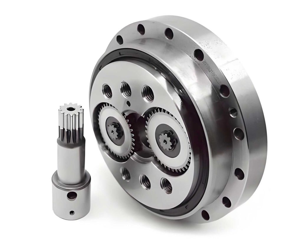
The RV reducer operates through a compound mechanism involving planetary gears and cycloid-pin transmissions, which are susceptible to various static and dynamic errors. Static errors arise from manufacturing and assembly tolerances, while dynamic errors result from time-varying stiffness, elastic deformations, and friction-induced wear. Over time, wear on the cycloid gear teeth alters the tooth profile, increasing backlash and reducing transmission accuracy. This wear process is gradual but cumulative, making it essential to model and predict its impact on reliability. In this study, I consider both static error sources and dynamic wear effects to build a comprehensive model for the RV reducer’s transmission accuracy. The goal is to optimize design parameters to maintain high reliability throughout the reducer’s operational life, thereby supporting the demand for robust and precise robotic systems.
Numerical Calculation and Prediction of Cycloid Gear Wear
Wear in the cycloid gear of an RV reducer primarily occurs due to sliding contact with the pins during meshing. To quantify this, I employ the Archard wear model, which relates wear volume to load, sliding distance, and material properties. The process involves calculating contact pressure, sliding distance, wear coefficient, and ultimately, wear depth. For an RV reducer under heavy loads, these calculations require iterative numerical methods due to the multi-tooth contact nature of cycloid-pin transmissions.
Contact Pressure Calculation
The contact pressure between the cycloid gear and pins is derived from meshing forces, which depend on the transmitted torque and tooth geometry. Given the complexity of multi-tooth engagement, I use a numerical approach. Initially, the maximum meshing force \( F_{\text{max}0} \) is estimated based on the torque \( T_c \), short width coefficient \( K_1 \), number of cycloid teeth \( z_c \), and pin circle radius \( r_p \):
$$ F_{\text{max}0} = \frac{4 T_c}{K_1 z_c r_p} $$
Using Hertzian contact theory, the deformation \( \delta_{\text{max}} \) at the point of maximum force is computed. For each meshing point \( i \) with phase angle \( \psi_i \), the meshing force \( F_i \) is assumed proportional to the difference between deformation \( \delta_i \) and initial backlash \( \Delta s_i \):
$$ F_i = \frac{F_{\text{max}}}{\delta_{\text{max}}} (\delta_i – \Delta s_i) $$
Meshing occurs only where \( \delta_i > \Delta s_i \), defining the engagement region. The torque balance equation for the cycloid gear is:
$$ T_c = \sum_{i=M}^{N} F_i l_i $$
where \( l_i \) is the distance from the meshing point’s normal to the gear center. Solving iteratively, the true maximum force \( F_{\text{max}} \) is obtained, and forces at other points are derived. The average contact pressure \( p_i \) at point \( i \) is then:
$$ p_i = \frac{F_i}{2b B} $$
Here, \( b \) is the contact half-width, and \( B \) is the gear width. This pressure distribution is crucial for wear calculations, as it varies along the tooth profile due to modification and wear progression.
Sliding Distance Determination
Relative sliding between the cycloid gear and pins contributes to wear. The sliding velocity \( v_r \) at a meshing point is given by:
$$ v_r = – \left( r_p \sqrt{s} – \sqrt{2} r_{rp} \right) \frac{\omega_H}{z_c} $$
where \( r_{rp} \) is the pin radius, \( s = 1 + K_1^2 – 2K_1 \cos \psi_i \), and \( \omega_H \) is the crankshaft angular velocity. The sliding coefficient \( \lambda \), representing the ratio of sliding to tangential velocity, is:
$$ \lambda = \frac{v_r}{v_t} $$
For a single engagement, the sliding distance \( du \) over the contact width is:
$$ du = 2b \lambda $$
This sliding distance accumulates over repeated cycles, leading to material removal.
Wear Coefficient Estimation
The wear coefficient \( k \) in the Archard model depends on material properties, lubrication, and surface conditions. Based on empirical regressions from wear experiments, I use the following formula to estimate \( k \):
$$ k = \frac{3.981 \times 10^{29}}{E’} L^{1.219} G^{-7.377} S^{1.589} $$
where \( E’ \) is the equivalent elastic modulus, and \( L \), \( G \), and \( S \) are dimensionless parameters for load, pressure-viscosity coefficient, and surface roughness, respectively:
$$ L = \frac{W’}{E’ R’}, \quad G = \alpha E’, \quad S = \frac{R_c^q}{\sqrt{R’}} $$
Here, \( W’ \) is the unit load, \( R’ \) is the equivalent curvature radius, \( \alpha \) is the pressure-viscosity coefficient, and \( R_c^q \) is the composite surface roughness. The wear coefficient is dynamic and influenced by operational conditions, but for this RV reducer analysis, I assume consistent lubrication and material pairs to simplify calculations.
Wear Depth Computation
Using the Archard model, the wear depth \( dh \) for a single engagement at point \( i \) is:
$$ dh = k p_i du $$
The meshing period \( t \), during which all teeth engage once, is:
$$ t = \frac{2\pi (z_p – 1)}{z_p \omega_H} $$
where \( z_p \) is the number of pins. Wear accumulates over time, and to account for changing contact pressures due to wear, I divide the process into \( Q \) intervals with reconstruction periods \( t_q \). The cumulative wear depth \( h_q \) in interval \( q \) is:
$$ h_q = \frac{1}{t} t_q dh $$
Total wear depth \( h \) over time \( T \) is:
$$ h = \sum_{q=1}^{Q} h_q $$
This iterative approach allows modeling progressive wear, though it is computationally intensive. For the RV reducer, modifications such as equidistant and shift modifications affect the meshing forces and wear distribution. I analyze various modification combinations to understand their impact on wear.
| Parameter | Value | Parameter | Value |
|---|---|---|---|
| Number of cycloid teeth, \( z_c \) | 39 | Shift modification, \( \Delta r_p \) (mm) | -0.030 |
| Number of pins, \( z_p \) | 40 | Elastic modulus (GPa) | 206 |
| Pin radius, \( r_{rp} \) (mm) | 5 | Poisson’s ratio | 0.3 |
| Pin circle radius, \( r_p \) (mm) | 114.5 | Sun gear pitch radius (mm) | 15 |
| Eccentricity, \( e \) (mm) | 2.2 | Center distance (mm) | 63 |
| Gear width, \( B \) (mm) | 18 | Pressure angle (°) | 20 |
| Equidistant modification, \( \Delta r_{rp} \) (mm) | -0.026 | Rated load, \( T_z \) (N·m) | 3136 |
For the RV reducer in Table 1, I explore modification ranges. The equidistant modification \( \Delta r_{rp} \) varies from -0.053 mm to 0.011 mm, with shift modification \( \Delta r_p \) adjusted to maintain initial radial clearance. Wear after 100 hours is computed for different combinations. Results show that larger equidistant modifications reduce maximum meshing forces and wear depth, leading to more uniform wear distribution along the tooth profile. This highlights the importance of modification parameters in managing wear for the RV reducer.
Wear Prediction Using Gaussian Process Regression
To reduce computational cost, I employ a Gaussian process regression model to predict wear based on limited simulation data. Wear is treated as a stochastic process following a normal distribution. The model uses input variables such as load \( T_z \), speed \( n \), time \( T \), and modification parameters, outputting predicted wear depth. The joint Gaussian distribution for observed wear \( w_o \) and predicted wear \( w_p \) is:
$$ \begin{bmatrix} w_o \\ w_p \end{bmatrix} \sim N \left( 0, \begin{bmatrix} K_{oo} + \sigma^2 I & K_{op} \\ K_{po} & K_{pp} \end{bmatrix} \right) $$
where \( K_{oo} \), \( K_{op} \), \( K_{po} \), and \( K_{pp} \) are covariance matrices, and \( \sigma^2 \) is noise variance. The predictive model is:
$$ w_p \sim N \left( K_{po}[K_{oo} + \sigma^2 I]^{-1} w_o, K_{pp} – K_{po}[K_{oo} + \sigma^2 I]^{-1} K_{op} \right) $$
Training on simulation data, this model accurately predicts wear, as validated by comparing predictions with simulations for the RV reducer under rated conditions. The Gaussian process approach enables efficient wear forecasting, essential for long-term reliability analysis.
Dynamic Reliability Model for Transmission Accuracy with Wear
The transmission accuracy of an RV reducer is quantified by backlash, which is influenced by both static errors and dynamic wear. I develop a reliability model that incorporates these factors to assess the probability that backlash remains within allowable limits over time.
Transmission Accuracy Model
Total backlash \( \Delta \phi \) in the RV reducer arises from various error sources, each contributing a normal backlash component \( \Delta \beta_j \). The formula for backlash in arcminutes is:
$$ \Delta \phi = \frac{180 \times 60}{\pi} \left( \sum_{j=1}^{3} \frac{\Delta \beta_j}{i_H r_1} + \sum_{j=4}^{15} \frac{\Delta \beta_j}{e z_c} + \frac{\Delta \beta_{16}}{a} \right) $$
where \( i_H \) is the reduction ratio, \( r_1 \) is the sun gear pitch radius, \( e \) is eccentricity, and \( a \) is center distance. The error factors include manufacturing tolerances, assembly clearances, and wear-induced changes. Wear on the cycloid gear adds an equivalent normal backlash similar to that from modifications. Table 2 summarizes error factors and their sensitivity indices, derived from partial derivatives of backlash with respect to each error.
| Error Factor | Normal Backlash Contribution | Sensitivity Index \( s_j \) |
|---|---|---|
| Gear tooth error, \( E_w \) | \( -E_w / \cos \theta \) | -0.037 |
| Pin circle radius error, \( \delta r_p \) | \( 2 \delta r_p \sqrt{1 – K_1^2} \) | 1.00 |
| Equidistant modification, \( \Delta r_{rp} \) | \( 2 \Delta r_{rp} \) | 1.56 |
| Shift modification, \( \Delta r_p \) | \( -2 \Delta r_p \sqrt{1 – K_1^2} \) | -1.00 |
| Cycloid gear wear, \( \delta w \) | \( 2 \delta w \) | 1.56 |
| Crankshaft bearing clearance, \( \Delta r \) | \( \Delta r \) | 1.06 |
Note: Only key errors are shown; others include pin radius error, assembly gaps, and profile deviations. The sensitivity index, normalized to pin circle radius error, indicates that modifications and wear have high impact on backlash in the RV reducer.
Dynamic Reliability Analysis
With wear progressing over time, backlash becomes a dynamic variable. The reliability function \( g(\mathbf{x}, \Delta \phi_{\text{per}}) \) defines the state where actual backlash \( \Delta \phi \) is less than permissible backlash \( \Delta \phi_{\text{per}} \):
$$ g(\mathbf{x}, \Delta \phi_{\text{per}}) = \Delta \phi_{\text{per}} – \Delta \phi $$
Here, \( \mathbf{x} = (T_z, n, T, \Delta r_{rp}, \Delta r_p) \) is the vector of operational and design parameters. Failure occurs if \( g < 0 \). Since errors and wear are random, I use Monte Carlo simulation to estimate reliability. For \( d \) samples of error values and wear depths at time \( T \), the number of failure samples \( d_T \) is counted. The time-dependent reliability \( R_T \) is:
$$ R_T = 1 – \frac{d_T}{d} $$
Assuming errors follow normal or Rayleigh distributions as per manufacturing data, I simulate backlash for the RV reducer under rated load (3136 N·m) and speed (15 rpm). Initially, without wear, backlash averages 0.7 arcminutes, below the allowable 1 arcminutes, indicating high reliability. However, as wear accumulates, reliability decreases. For instance, at 6,000 hours, reliability drops to 88.7%, which may be insufficient for precision applications. This underscores the need for parameter optimization to sustain reliability over the RV reducer’s lifespan.
Sensitivity Analysis of Error Factors
To prioritize optimization efforts, I conduct a sensitivity analysis by computing partial derivatives of backlash with respect to each error factor. The sensitivity vector \( \mathbf{S} \) is:
$$ \mathbf{S} = \left( \frac{\partial \Delta \phi}{\partial \Delta \phi_1}, \frac{\partial \Delta \phi}{\partial \Delta \phi_2}, \dots, \frac{\partial \Delta \phi}{\partial \Delta \phi_{16}} \right) $$
Using the pin circle radius error as reference, sensitivity indices \( s_j \) are derived as ratios. High-index errors, such as those from modifications and wear, significantly influence backlash and thus are focus areas for optimizing the RV reducer.
Multi-Objective Optimization of Parameters
I formulate a multi-objective optimization problem to minimize machining cost and maximum wear over the rated life, subject to reliability constraints. Design variables include tolerances for key components and modification parameters for the cycloid gear.
Optimization Model
The objective functions are:
$$ \min \, F(\mathbf{E}) = [C(\mathbf{E}_i), W(\mathbf{E}_j)] $$
where \( C(\mathbf{E}_i) \) is total machining cost for tolerances \( \mathbf{E}_i \), and \( W(\mathbf{E}_j) \) is maximum wear depth over 6,000 hours for modification parameters \( \mathbf{E}_j \). Cost functions for different tolerance types are based on empirical models:
For size tolerances:
$$ C_1(E_i) = a_1 e^{-a_2 E_i} + \frac{a_5}{a_3 E_i + a_4} $$
with coefficients \( a_1 = 16.140, a_2 = 0.324, a_3 = 0.217, a_4 = 0.013, a_5 = 2.845 \).
For position tolerances:
$$ C_2(E_i) = b_1 e^{-b_2 E_i} + \frac{b_3}{E_i^{b_4}} $$
with \( b_1 = 4.862, b_2 = 0.483, b_3 = 0.877, b_4 = 1.020 \).
For runout tolerances:
$$ C_3(E_i) = c_1 e^{-c_2 E_i} $$
with \( c_1 = 23.729, c_2 = 0.682 \).
Total cost \( C \) is the sum of these functions. The constraint ensures reliability at 6,000 hours meets a target \( R_{\text{per}} \):
$$ R_T(\mathbf{x}, \Delta \phi_{\text{per}}) \geq R_{\text{per}} $$
I consider two cases: \( R_{\text{per}} = 95\% \) and \( R_{\text{per}} = 100\% \). Design variable ranges are set based on practical machining limits, as shown in Table 3.
| Variable | Lower Bound (mm) | Upper Bound (mm) |
|---|---|---|
| Equidistant modification, \( \Delta r_{rp} \) | -0.053 | 0.011 |
| Shift modification, \( \Delta r_p \) | -0.057 | 0.007 |
| Pin circle radius tolerance, \( \delta r_p \) | 0.0025 | 0.005 |
| Pin radius tolerance, \( \delta r_{rp} \) | -0.010 | -0.006 |
| Assembly clearance, \( \delta J \) | 0.005 | 0.020 |
Other variables include profile errors and runout tolerances, with bounds derived from manufacturing standards.
Optimization Results
Using a genetic algorithm, I obtain Pareto-optimal solutions for both reliability constraints. The Pareto fronts trade off cost and wear, with knee points selected as optimal compromises. Table 4 presents optimized parameters for the two cases.
| Parameter | Optimized for 95% Reliability | Optimized for 100% Reliability |
|---|---|---|
| \( \Delta r_{rp} \) (mm) | -0.0287 | -0.0347 |
| \( \Delta r_p \) (mm) | -0.0327 | -0.0387 |
| \( \delta r_p \) (mm) | ±0.0045 | ±0.0041 |
| \( \delta r_{rp} \) (mm) | -0.0062 | -0.0073 |
| \( \delta J \) (mm) | \(^{+0.0130}_{-0.0082}\) | \(^{+0.0151}_{-0.0084}\) |
| Maximum wear at 6,000 h (μm) | 3.151 | 3.207 |
| Machining cost (monetary units) | 1291 | 1300 |
Compared to initial values (wear 3.127 μm, cost 1402), optimization reduces cost by 7.9% and 7.3% for the two cases, with slight wear increases of 0.77% and 2.56%, respectively. The reliability curves show that optimized RV reducers maintain reliability above 95% or 100% over 6,000 hours, meeting design targets. This demonstrates that careful parameter selection can enhance the RV reducer’s performance while controlling costs.
Discussion and Implications
The analysis reveals that wear significantly impacts the transmission accuracy reliability of RV reducers, even when initial backlash is within limits. The dynamic reliability model, incorporating wear predictions, provides a realistic assessment over time. Optimization results highlight trade-offs: stricter reliability constraints (e.g., 100%) require tighter tolerances and modifications, increasing cost marginally, but still offer savings compared to initial designs. The Gaussian process regression proves effective for wear prediction, reducing computational burden in reliability simulations.
For practical applications, this approach allows designers to tailor RV reducers for specific reliability requirements. For instance, in high-precision robotics, targeting 100% reliability may be justified, whereas cost-sensitive applications might opt for 95% with lower expenses. The sensitivity analysis guides focus on critical parameters, such as modifications and wear management, which are key to maintaining RV reducer accuracy.
Conclusion
In this study, I developed a comprehensive framework for analyzing and optimizing the transmission accuracy reliability of an RV reducer considering cycloid gear wear. By integrating wear calculations via the Archard model, backlash modeling, and dynamic reliability assessment, I demonstrated how wear progressively degrades performance. The multi-objective optimization balanced machining cost and wear minimization under reliability constraints, yielding parameter sets that enhance RV reducer longevity and precision. Results confirm that optimized designs can achieve desired reliability levels over a 6,000-hour lifespan with reduced costs, offering valuable insights for the development of high-performance RV reducers in robotic and industrial applications. Future work could explore real-time wear monitoring or adaptive lubrication strategies to further improve RV reducer reliability.