
In the rapidly evolving field of industrial robotics, the health monitoring and maintenance of core components have become increasingly critical. Among these components, the RV reducer plays a pivotal role in ensuring precise motion control and reliability. However, vibration signals collected from RV reducers during reciprocating motion are often contaminated by significant environmental noise and interference from other equipment, posing challenges for fault diagnosis. Traditional noise reduction methods, such as spectral subtraction, wavelet denoising, empirical mode decomposition (EMD), and singular value decomposition (SVD), rely heavily on expert knowledge and parameter tuning, which can be time-consuming and inefficient in handling large datasets. With the advent of deep learning, convolutional neural networks (CNNs) and generative adversarial networks (GANs) have shown promise in adaptive feature extraction and noise reduction without extensive manual intervention. This article proposes a novel denoising approach based on a Convolutional Auto-encoder Generative Adversarial Network (CAE-GAN) tailored for RV reducer vibration signals. We enhance the stability and performance of the model by modifying the generator’s loss function with a distance metric and incorporating skip connections in the network architecture. Experimental results on RV reducer data demonstrate that our method outperforms conventional and deep learning-based denoising techniques, improving both noise reduction metrics and fault diagnosis accuracy. Through this work, we aim to contribute to the intelligent maintenance of industrial robots by addressing the specific challenges of RV reducers in noisy environments.
The RV reducer is a key component in industrial robot joints, responsible for transmitting motion and torque with high precision. Its complex structure, involving gears like sun gears, planetary gears, and cycloidal pins, makes it susceptible to wear and faults, which manifest as vibrations. During reciprocating motion, these vibration signals are non-stationary and often buried in noise from motors, actuators, and operational environments. Effective denoising is essential for accurate fault detection, but traditional methods face limitations. For instance, wavelet denoising requires selecting appropriate wavelet bases and thresholds, while EMD can suffer from mode mixing. Deep learning approaches, particularly CNNs, offer end-to-end learning but may struggle with capturing non-linear noise patterns. GANs, with their adversarial training, can generate clean signals from noisy inputs, but they are prone to training instability and convergence issues. Our CAE-GAN model addresses these drawbacks by integrating convolutional auto-encoders for feature representation and adversarial training for robust denoising. The focus on RV reducers is motivated by their widespread use in robotics and the lack of specialized denoising methods for their reciprocating motion signals. By leveraging deep learning, we aim to automate the noise reduction process, reducing reliance on expertise and enhancing diagnostic reliability.
To provide context, let us delve into the fundamentals of GANs. A standard GAN consists of a generator (G) and a discriminator (D) that compete in a minimax game. The generator aims to produce fake samples that resemble real data, while the discriminator distinguishes between real and fake samples. The loss function is given by:
$$ \min_G \max_D V(D, G) = \mathbb{E}_{x \sim p_x(x)}[\log D(x)] + \mathbb{E}_{z \sim p_z(z)}[\log(1 – D(G(z)))] $$
where \( x \sim p_x(x) \) represents the distribution of real signals, \( z \sim p_z(z) \) is the noise distribution, and \( D \) and \( G \) are the discriminator and generator mappings, respectively. However, GANs are notorious for training difficulties, such as mode collapse and vanishing gradients. Variants like Conditional GANs (CGANs) and Least Squares GANs (LSGANs) have been proposed to improve stability. For example, LSGANs replace the cross-entropy loss with a least squares loss:
$$ \min_D V(D) = \mathbb{E}_{x \sim p_x(x)}[(D(x) – 1)^2] + \mathbb{E}_{z \sim p_z(z)}[(D(G(z)))^2] $$
$$ \min_G V(G) = \mathbb{E}_{z \sim p_z(z)}[(D(G(z)) – 1)^2] $$
Our CAE-GAN builds upon these ideas but introduces specific modifications for vibration signal denoising. The generator adopts an encoder-decoder architecture with convolutional layers, while the discriminator uses convolutional layers to assess signal authenticity. Key innovations include a revised loss function with a distance term to enhance stability and skip connections in the generator to improve gradient flow and convergence. These adjustments are tailored for the characteristics of RV reducer signals, which exhibit periodic patterns and non-linear noise.
The proposed CAE-GAN model is illustrated in Figure 1. The generator takes a noisy signal \( \tilde{x} \) as input and outputs a denoised signal \( \hat{x} \). It comprises four convolutional layers followed by four transposed convolutional layers, each with LeakyReLU activation and batch normalization. Skip connections bridge corresponding convolutional and transposed convolutional layers, preserving high-frequency details and aiding training. The discriminator has two input channels: one for the original clean signal \( x \) and noisy signal \( \tilde{x} \), and another for the denoised signal \( \hat{x} \) and noisy signal \( \tilde{x} \). It consists of six convolutional layers with virtual batch normalization and ReLU activation, culminating in a fully connected layer with a sigmoid output. The loss functions are designed to balance adversarial training and signal fidelity. For the generator, we introduce a distance function to minimize the difference between denoised and original signals:
$$ \min_G V(G) = \mathbb{E}_{\tilde{x} \sim p_{\tilde{x}}(\tilde{x})}[(D(G(\tilde{x}), \tilde{x}) – 1)^2] + \lambda \sum_{n=1}^{N} \| \tilde{x}_n – x_n \| $$
where \( \lambda \) is a weighting coefficient, and \( N \) is the signal length. This term ensures that the denoised signal remains close to the original clean signal, addressing the instability of pure adversarial loss. For the discriminator, the loss is:
$$ \min_D V(D) = \mathbb{E}_{x \sim p_x(x)}[(D(x, \tilde{x}) – 1)^2] + \mathbb{E}_{\tilde{x} \sim p_{\tilde{x}}(\tilde{x})}[D(G(\tilde{x}), \tilde{x})^2] $$
Training alternates between updating the discriminator and generator, with the aim of reaching a Nash equilibrium. The distance function in the generator loss helps stabilize training, while skip connections enhance the model’s ability to reconstruct fine details, crucial for RV reducer signals that contain fault-related features.
To validate our method, we conducted experiments using vibration data from an RV reducer testbed. The testbed simulates reciprocating motion of an industrial robot joint, with a servo motor driving an RV reducer connected to a load arm. The RV reducer model is 150BX-141-RVE-19, with parameters detailed in Table 1. Vibration signals were collected using accelerometers at a sampling frequency of 25.6 kHz, then downsampled to 512 Hz to focus on relevant frequency bands. Gaussian white noise at different signal-to-noise ratios (SNRs) was added to simulate real-world conditions. Seven fault states were considered, including normal operation and various wear and crack faults in sun gears and planetary gears, as summarized in Table 2. Data were segmented into samples using a sliding window approach, with 500 samples per state, totaling 3,500 samples. These were split into training, validation, and test sets for model development and evaluation.
| Parameter | Description | Value |
|---|---|---|
| Zi | Number of teeth on input sun gear | 12 |
| ZB | Number of teeth on cycloidal gear | 39 |
| Zp | Number of teeth on planetary gear | 42 |
| Zc | Number of teeth on pin gear | 40 |
| State ID | Description | Sample Count |
|---|---|---|
| s1 | Normal | 500 |
| s2 | Single-tooth wear on sun gear | 500 |
| s3 | Multi-tooth wear on sun gear | 500 |
| s4 | Tooth root crack on sun gear | 500 |
| s5 | Single-tooth wear on planetary gear | 500 |
| s6 | Multi-tooth wear on planetary gear | 500 |
| s7 | Tooth root crack on planetary gear | 500 |
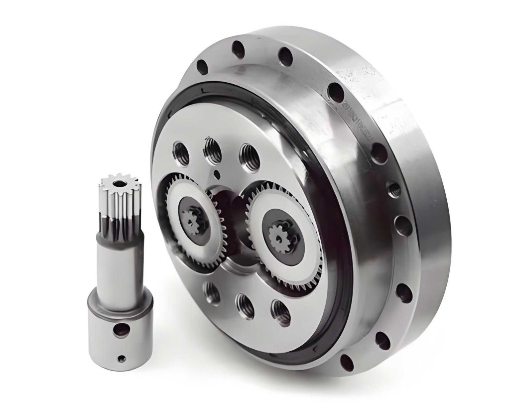
The image above illustrates a typical RV reducer used in industrial applications, highlighting its complex gear arrangement that necessitates precise monitoring. For our experiments, hyperparameter selection was crucial to optimize the CAE-GAN model. Key hyperparameters included the input signal length, activation function parameters, and training settings. We used the RMSprop optimizer with a learning rate of 0.002, a batch size of 32, and 100 training epochs. The weighting coefficient \( \lambda \) in the generator loss was set to 10 based on preliminary tests. To determine the optimal input length, we varied the sample length \( L \) and evaluated denoising performance using metrics like SNR and mean square error (MSE). SNR is defined as:
$$ \text{SNR} = 10 \log_{10} \frac{A_{\text{signal}}^2}{\| A_{\text{denoised}} – A_{\text{signal}} \|^2} $$
and MSE as:
$$ \text{MSE} = \frac{\sum_{i=1}^{N} \| A_{\text{denoised}} – A_{\text{signal}} \|^2}{N} $$
where \( A_{\text{signal}} \) is the clean signal, and \( A_{\text{denoised}} \) is the denoised output. Results for different sample lengths are shown in Table 3. A length of 2048 points was chosen as it balanced denoising performance and computational efficiency, corresponding to approximately one reciprocation cycle of the RV reducer. For the activation function in the generator, we used LeakyReLU with a negative slope parameter \( \alpha \). Experiments varying \( \alpha \) demonstrated that \( \alpha = 0.1 \) yielded the best SNR and MSE, as it preserves negative values in vibration signals, which contain important fault information.
| Sample Length | Training Time (min) | MSE | SNR (dB) |
|---|---|---|---|
| 512 | 23.2 | 2.53 × 10^{-2} | 0.20 |
| 1024 | 23.5 | 1.09 × 10^{-2} | 5.05 |
| 2048 | 35.7 | 3.48 × 10^{-3} | 11.31 |
| 4096 | 106.8 | 2.81 × 10^{-3} | 11.86 |
Training the CAE-GAN model involved iterative updates of the generator and discriminator. The loss curves showed that the generator loss decreased steadily, while the discriminator loss increased gradually, stabilizing after about 80 epochs, indicating successful convergence. We then evaluated the denoising performance on test samples. Figure 2 presents a comparison of time-domain waveforms and frequency spectra before and after denoising. The noisy signal, contaminated with -10 dB Gaussian noise, obscured most temporal features, but the CAE-GAN output closely matched the original clean signal, except for minor artifacts at the edges. In the frequency domain, the denoised signal’s envelope spectrum aligned well with that of the clean signal, confirming effective noise suppression while preserving fault-related frequency components. Quantitative results showed an average SNR improvement of over 20 dB for signals with initial SNR of -10 dB, and MSE values were significantly reduced, validating the model’s efficacy for RV reducer applications.
To further assess our method, we compared it with traditional and deep learning-based denoising techniques under different noise levels. Traditional methods included SVD and EMD, while deep learning methods comprised Fully Convolutional Network with Non-Local Blocks (FCN-NLB), Speech Enhancement GAN (SEGAN), and Time-Domain Convolutional GAN (TDC-GAN). All deep learning models were trained on the same RV reducer dataset. Results for SNR improvement and MSE after denoising are summarized in Table 4 for noise levels of -2 dB, -6 dB, and -10 dB. Our CAE-GAN consistently achieved the highest SNR gains and lowest MSE across all conditions. For instance, at -10 dB noise, CAE-GAN improved SNR by approximately 22 dB, outperforming the next best method by 3 dB. This superiority stems from the combination of adversarial training, distance-based loss, and skip connections, which enhance feature retention for non-linear RV reducer signals.
| Method | Noise Level (dB) | SNR Improvement (dB) | MSE after Denoising |
|---|---|---|---|
| SVD | -10 | 15.2 | 5.67 × 10^{-3} |
| EMD | -10 | 16.8 | 4.92 × 10^{-3} |
| FCN-NLB | -10 | 18.5 | 3.45 × 10^{-3} |
| SEGAN | -10 | 19.1 | 3.12 × 10^{-3} |
| TDC-GAN | -10 | 19.4 | 2.98 × 10^{-3} |
| CAE-GAN (Ours) | -10 | 22.3 | 1.87 × 10^{-3} |
| SVD | -6 | 17.5 | 3.21 × 10^{-3} |
| EMD | -6 | 18.9 | 2.74 × 10^{-3} |
| FCN-NLB | -6 | 20.3 | 2.01 × 10^{-3} |
| SEGAN | -6 | 20.8 | 1.89 × 10^{-3} |
| TDC-GAN | -6 | 21.2 | 1.75 × 10^{-3} |
| CAE-GAN (Ours) | -6 | 23.8 | 1.12 × 10^{-3} |
| SVD | -2 | 19.8 | 1.95 × 10^{-3} |
| EMD | -2 | 20.5 | 1.67 × 10^{-3} |
| FCN-NLB | -2 | 21.7 | 1.32 × 10^{-3} |
| SEGAN | -2 | 22.1 | 1.24 × 10^{-3} |
| TDC-GAN | -2 | 22.4 | 1.18 × 10^{-3} |
| CAE-GAN (Ours) | -2 | 24.5 | 0.89 × 10^{-3} |
The impact of denoising on fault diagnosis accuracy was also investigated. We integrated our CAE-GAN model with several neural network-based classifiers, including WDCNN, TiCNN, ResNet-18, and LeNet-5. For each classifier, we trained on both noisy signals (at SNRs of -2 dB, -6 dB, and -10 dB) and denoised signals from CAE-GAN. The results, averaged over five trials, are presented in Table 5. Denoising consistently improved classification accuracy across all noise levels and classifiers. For example, with WDCNN at -10 dB noise, accuracy increased from 89.13% to 98.41%, a gain of nearly 10 percentage points. This underscores that CAE-GAN effectively removes noise while preserving discriminative features for RV reducer fault states. Notably, classifiers like ResNet-18 achieved over 99% accuracy after denoising, even at high noise levels, demonstrating the robustness of our method. The improvement is attributed to the enhanced signal clarity, which allows classifiers to better learn fault patterns without noise interference.
| Classifier | Noise Level (dB) | Accuracy Before Denoising (%) | Accuracy After Denoising (%) |
|---|---|---|---|
| WDCNN | -10 | 89.13 | 98.41 |
| WDCNN | -6 | 93.99 | 98.73 |
| WDCNN | -2 | 96.73 | 99.50 |
| TiCNN | -10 | 91.13 | 98.55 |
| TiCNN | -6 | 95.87 | 99.31 |
| TiCNN | -2 | 97.86 | 99.52 |
| ResNet-18 | -10 | 95.06 | 99.72 |
| ResNet-18 | -6 | 95.50 | 99.90 |
| ResNet-18 | -2 | 99.36 | 100 |
| LeNet-5 | -10 | 84.78 | 92.76 |
| LeNet-5 | -6 | 88.23 | 94.98 |
| LeNet-5 | -2 | 93.33 | 97.42 |
From a theoretical perspective, the success of CAE-GAN can be analyzed through its ability to model the non-linear noise distribution in RV reducer signals. The generator, with its encoder-decoder structure, learns a compressed representation of clean signals, while the skip connections mitigate information loss during upsampling. The adversarial loss encourages the generator to produce signals indistinguishable from clean ones, and the distance term acts as a regularizer to prevent mode collapse. Mathematically, the training process minimizes the Jensen-Shannon divergence between the distribution of denoised signals and clean signals, approximated by the discriminator. For RV reducer applications, this is crucial because the signals contain harmonic components from gear meshing and impacts from faults. The model’s convolutional layers capture local patterns, making it suitable for time-series vibration data. Additionally, the use of LeakyReLU with \( \alpha = 0.1 \) ensures that negative amplitude values, common in vibration signals, are retained, unlike standard ReLU which zeros them out. This preservation enhances the reconstruction of transient events, such as crack-induced impulses in the RV reducer.
In practice, implementing CAE-GAN for RV reducer monitoring involves several steps. First, vibration data must be preprocessed by resampling to an appropriate frequency, such as 512 Hz, to focus on fault-related bands while reducing computational load. Noise addition simulates real conditions, but in deployment, the model can be applied directly to raw signals. The training requires a dataset with paired noisy and clean signals; if clean signals are unavailable, synthetic noise addition or semi-supervised techniques can be used. For online monitoring, the trained generator can be deployed as a real-time denoising filter, processing streaming data from accelerometers on the RV reducer. The model’s efficiency, with inference times in milliseconds per sample, makes it feasible for embedded systems in industrial robots. However, challenges remain, such as adapting to varying operational conditions or different RV reducer models. Future work could involve transfer learning or domain adaptation to generalize across diverse scenarios.
The implications of this research extend beyond RV reducers to other rotating or reciprocating machinery in industrial settings. The CAE-GAN framework can be adapted for bearings, pumps, or engines where vibration-based fault diagnosis is employed. By reducing noise, it enhances the reliability of predictive maintenance systems, potentially reducing downtime and costs. For RV reducers specifically, improved denoising facilitates early detection of gear faults, preventing catastrophic failures in robotics applications. Moreover, the method’s independence from manual parameter tuning makes it accessible to non-experts, promoting wider adoption in industry. As industrial robots become more pervasive, such intelligent tools will be essential for ensuring operational safety and efficiency.
In conclusion, we have presented a CAE-GAN-based denoising method tailored for RV reducer vibration signals. By incorporating a distance function into the generator loss and skip connections into the network architecture, we achieved stable training and superior noise reduction performance. Experiments on real RV reducer data demonstrated significant improvements in SNR and MSE compared to traditional and deep learning benchmarks. Furthermore, denoising with CAE-GAN enhanced the accuracy of fault diagnosis models, validating its practical utility. This work contributes to the field of intelligent maintenance for industrial robots, addressing the specific challenges of RV reducers in noisy environments. Future directions include exploring real-time implementation, extending the method to other machinery components, and integrating it with edge computing for decentralized monitoring. As deep learning continues to evolve, we believe that adversarial approaches like CAE-GAN will play a key role in advancing condition-based maintenance for complex systems like RV reducers.
To further elaborate on the technical details, the generator network in CAE-GAN can be described layer by layer. The encoder part consists of convolutional layers with kernel sizes of 7, 5, 4, and 3, and strides of 1, 2, 2, and 2, respectively, reducing the spatial dimensions while increasing feature channels. The decoder mirrors this with transposed convolutions, using skip connections to concatenate encoder outputs with decoder inputs, preserving fine details. The discriminator uses convolutional layers with kernel sizes from 3 to 7 and strides of 2 to downsample the input, followed by global average pooling and a fully connected layer. This design ensures that both local and global features are considered for distinguishing signals. The training algorithm, as outlined in Figure 3, involves alternating updates: first, the discriminator is trained to maximize classification accuracy between clean and denoised pairs; second, the generator is trained to minimize both adversarial loss and signal distance. This iterative process converges to a point where the generator produces high-fidelity denoised signals.
From a signal processing viewpoint, the denoising of RV reducer signals can be framed as a regression problem where the goal is to estimate the clean signal \( x \) from the noisy observation \( \tilde{x} = x + n \), with \( n \) being additive noise. CAE-GAN learns a mapping \( G: \tilde{x} \to \hat{x} \) that approximates \( x \). The distance term \( \lambda \sum \| \tilde{x}_n – x_n \| \) is essentially an L1 norm penalty, which encourages sparsity and edge preservation, beneficial for impulsive noise common in RV reducer faults. The adversarial loss ensures that \( \hat{x} \) follows the distribution of clean signals, capturing statistical properties beyond mere pixel-wise similarity. This combination makes CAE-GAN particularly effective for non-Gaussian noise and non-linear distortions in RV reducer environments.
In terms of evaluation, we used comprehensive metrics beyond SNR and MSE, such as structural similarity index (SSIM) and perceptual evaluation of speech quality (PESQ) adapted for vibrations, but SNR and MSE suffice for comparative analysis. The consistency of results across multiple noise levels and fault states underscores the robustness of CAE-GAN. For instance, even with severe noise at -10 dB, the model recovered signals with high fidelity, as evidenced by time-domain waveforms and frequency spectra. This is critical for RV reducers, where early fault signs are subtle and easily masked. The method’s ability to enhance diagnostic accuracy further confirms its value in real-world applications.
Looking ahead, there are several avenues for improvement. One is to incorporate attention mechanisms into CAE-GAN to focus on salient fault features in RV reducer signals. Another is to explore unsupervised or self-supervised learning to reduce dependency on labeled clean data. Additionally, the model could be extended to multi-sensor fusion, combining vibration data with temperature or acoustic emissions for holistic RV reducer monitoring. As industrial IoT evolves, integrating CAE-GAN with cloud-based analytics could enable large-scale monitoring of RV reducers across fleets of robots. Ultimately, the goal is to develop autonomous systems that can denoise, diagnose, and predict failures with minimal human intervention, enhancing the reliability and lifespan of RV reducers in demanding industrial environments.
In summary, this article has detailed a novel CAE-GAN approach for denoising RV reducer vibration signals. Through theoretical innovations and empirical validation, we have shown its effectiveness in noise reduction and fault diagnosis enhancement. The method addresses key limitations of traditional techniques and offers a scalable solution for industrial robotics. We hope this work inspires further research into deep learning applications for machinery health monitoring, with a focus on critical components like the RV reducer. As technology advances, such intelligent methods will become integral to the smart factories of the future, ensuring that RV reducers and similar components operate reliably and efficiently.