
The quest for robust and reliable autonomous navigation represents one of the fundamental challenges in robotics. At the heart of this challenge lies the Simultaneous Localization and Mapping (SLAM) problem, where an embodied AI robot must concurrently construct a model of its unknown environment while estimating its own position within it. Traditional SLAM pipelines, often reliant on a single primary sensor like a LiDAR or a camera, struggle with the inherent limitations and failure modes of their chosen modality—be it feature scarcity for LiDAR in long corridors or illumination sensitivity for cameras. This brittleness is unacceptable for an embodied AI robot operating in the dynamic, unstructured, and complex real world, where its survival and success depend on continuous, reliable spatial awareness.
The paradigm of embodied AI shifts the perspective from passive perception to active, situated interaction. An embodied AI robot is not merely a passive observer but an agent whose intelligence is fundamentally shaped by its physical structure, its sensors, and its dynamic coupling with the environment. This perspective is crucial for SLAM. It demands algorithms that do not just process data but actively leverage multi-modal sensory streams, adapt to contextual changes, and utilize the robot’s own motion to disambiguate perception. This work presents the research and implementation of a multi-source fusion SLAM algorithm, architected from the ground up with the principles of embodied intelligence. Our system integrates LiDAR, visual cameras, an Inertial Measurement Unit (IMU), and wheel encoders, fusing their asynchronous data streams within a deep learning-enhanced framework. We demonstrate how this embodied AI approach enables an autonomous vehicle—a prime example of a complex embodied AI robot—to achieve superior localization accuracy, map consistency, and operational robustness in challenging outdoor environments.
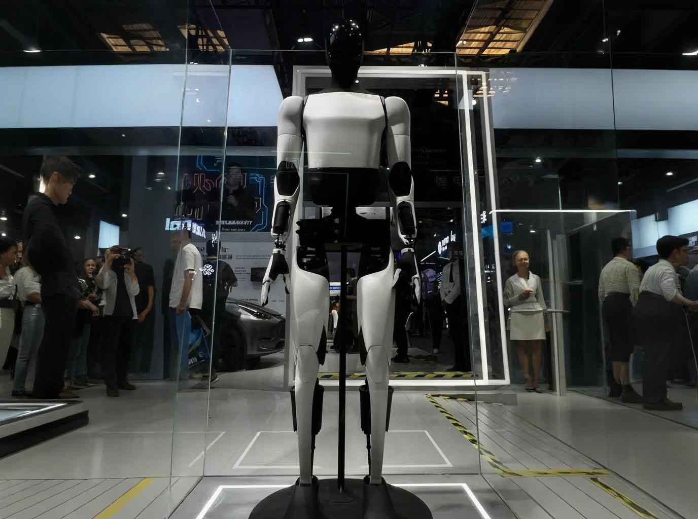
The core thesis is that a truly intelligent embodied AI robot must perform sensor fusion not as an afterthought but as a foundational, tightly-coupled process. The robot’s “body”—its sensor suite and kinematic model—provides complementary constraints that, when properly modeled and optimized, resolve the ambiguities that plague single-sensor systems. The subsequent sections detail our architecture, beginning with the sensor suite and fusion strategy, proceeding through the front-end odometry, back-end optimization, and loop closure mechanisms, all reinforced by targeted deep learning modules, and concluding with experimental validation.
1. The Embodied Sensor Suite and State Estimation
The perceptual foundation of our embodied AI robot is a heterogeneous array of sensors, each chosen for its complementary strengths and weaknesses. The key to robust state estimation for an embodied AI robot lies in explicit modeling of these characteristics and their synergistic fusion. The table below summarizes the role and error characteristics of each sensor in our system.
| Sensor | Measurement | Role in State Estimation | Primary Error Characteristics |
|---|---|---|---|
| 3D LiDAR | High-resolution 3D point clouds | Provides precise 6-DoF motion estimation via scan matching. Primary source for map geometry. | Motion distortion; degeneracy in feature-less environments (e.g., tunnels, flat walls). |
| Stereo/RGB Cameras | Sequential image frames | Provides rich texture and feature data. Crucial for estimating vertical motion and aiding visual odometry. | Highly sensitive to lighting changes, motion blur, and low-texture scenes. |
| Inertial Measurement Unit (IMU) | 3-axis angular velocity & linear acceleration | Provides high-frequency ego-motion prediction between low-frequency LiDAR/Camera frames. Critical for motion de-distortion. | Suffers from bias, noise, and significant drift due to double integration over time. |
| Wheel Encoders | Wheel rotation counts | Provides planar (2D) odometry, offering a reliable, low-drift estimate of longitudinal displacement on flat ground. | Susceptible to wheel slip, terrain deformation, and calibration errors. Provides only 2D information. |
The state of the embodied AI robot at time \( k \) is represented as \( \mathbf{x}_k = [\mathbf{p}_k, \mathbf{q}_k, \mathbf{v}_k, \mathbf{b}_k^a, \mathbf{b}_k^g] \), where \( \mathbf{p}_k \in \mathbb{R}^3 \) is position, \( \mathbf{q}_k \in \mathbb{SO}(3) \) is orientation (quaternion), \( \mathbf{v}_k \in \mathbb{R}^3 \) is velocity, and \( \mathbf{b}_k^a, \mathbf{b}_k^g \) are IMU acceleration and gyroscope biases. The goal of front-end estimation is to propagate this state using all available sensor data.
The IMU provides a direct but noisy prediction. The kinematic model between two IMU measurements at times \( i \) and \( j \) is:
$$
\begin{aligned}
\mathbf{p}_j &= \mathbf{p}_i + \mathbf{v}_i \Delta t + \iint_{t \in [i, j]} (\mathbf{R}_t (\tilde{\mathbf{a}}_t – \mathbf{b}_t^a) – \mathbf{g}) dt^2 \\
\mathbf{v}_j &= \mathbf{v}_i + \int_{t \in [i, j]} (\mathbf{R}_t (\tilde{\mathbf{a}}_t – \mathbf{b}_t^a) – \mathbf{g}) dt \\
\mathbf{q}_j &= \mathbf{q}_i \otimes \int_{t \in [i, j]} \frac{1}{2} \boldsymbol{\Omega}(\tilde{\boldsymbol{\omega}}_t – \mathbf{b}_t^g) \mathbf{q}_t dt
\end{aligned}
$$
where \( \tilde{\mathbf{a}}_t \) and \( \tilde{\boldsymbol{\omega}}_t \) are raw IMU measurements, \( \mathbf{g} \) is gravity, \( \otimes \) denotes quaternion multiplication, and \( \boldsymbol{\Omega}(\cdot) \) forms a quaternion derivative matrix. This prediction, while high-frequency, drifts quickly. The role of the embodied AI robot‘s other sensors is to provide frequent, absolute measurements to correct this drift.
2. Deep Learning for Embodied Perception Enhancement
To address specific perceptual challenges faced by an embodied AI robot in dynamic environments, we integrate two targeted deep learning modules. These are not monolithic “black-box” networks but specialized tools that augment the geometric SLAM pipeline.
2.1 Dynamic Object Culling from LiDAR Point Clouds
Dynamic objects (vehicles, pedestrians) introduce moving landmarks that corrupt the static map and induce errors in scan matching and loop closure. An embodied AI robot must distinguish between the static world (the map) and transient entities. We employ a 3D object detection network based on a voxel-based architecture similar to CenterPoint. The process transforms a raw point cloud \( \mathcal{P} = \{\mathbf{p}_i\} \) into a set of detected dynamic object bounding boxes \( \mathcal{B} = \{ \mathbf{b}_j \} \), where \( \mathbf{b}_j = [x, y, z, l, w, h, \theta, s] \) represents center, dimensions, yaw, and confidence score.
The network is trained with a loss function that combines localization and classification losses. A key component is the IoU-guided score target, which aligns confidence with localization quality:
$$
\text{IoU-Guided Target: } I_j = \min[1, \max(0, 2 \times \text{IoU}_j – 0.5)]
$$
$$
\text{Score Loss: } \mathcal{L}_{\text{score}} = -\frac{1}{N} \sum_{j=1}^{N} \left[ w \cdot I_j \log(\hat{s}_j) + (1 – I_j) \log(1 – \hat{s}_j) \right]
$$
Here, \( \text{IoU}_j \) is the intersection-over-union between the \( j\)-th proposal and its ground truth, \( \hat{s}_j \) is the predicted score, and \( w \) is a weight to balance positive and negative samples. All points within the high-confidence bounding boxes \( \mathcal{B} \) are filtered out before the point cloud \( \mathcal{P}’ \) is passed to the SLAM front-end, resulting in a map of only static structures.
2.2 Robust Visual Feature Matching with Descriptor Optimization
Visual odometry provides vital constraints, especially for vertical motion estimation where LiDAR is weak. Traditional hand-crafted features like ORB can fail under significant viewpoint or illumination changes. We design a learned feature matching system that produces more uniformly distributed and robust features. Given an image \( \mathbf{I} \), a dense feature map \( \mathbf{F} = f_{\text{CNN}}(\mathbf{I}) \) is extracted. For a keypoint at pixel location \( (u,v) \), its descriptor \( \mathbf{d} \) is sampled from \( \mathbf{F} \).
We optimize the descriptor space using a contrastive loss framework. For a pair of images \( \mathbf{I}_A, \mathbf{I}_B \) with a set of matched keypoint pairs \( \mathcal{M} = \{(i, j)\} \) and non-matched pairs \( \mathcal{N} \), the loss encourages matching descriptors to be close and non-matching ones to be distant:
$$
\mathcal{L}_{\text{desc}} = \sum_{(i,j) \in \mathcal{M}} \|\mathbf{d}_A^i – \mathbf{d}_B^j\|_2^2 + \sum_{(i,j) \in \mathcal{N}} \max(0, \alpha – \|\mathbf{d}_A^i – \mathbf{d}_B^j\|_2)^2
$$
where \( \alpha \) is a margin. This learned model, integrated into the embodied AI robot‘s vision pipeline, yields more reliable feature tracks across frames, improving the robustness of visual odometry estimates, particularly in challenging lighting conditions where the embodied AI robot must adapt.
3. Front-End Estimation: Tightly-Coupled Odometry
The front-end is responsible for computing a high-frequency, locally accurate odometry estimate. Our system implements a tightly-coupled scheme that fuses information at the measurement level.
Step 1: Incremental Pose Prior. Between two LiDAR scan times \( t_k \) and \( t_{k+1} \), we compute an incremental prior \( \Delta \tilde{\mathbf{x}}_{k \rightarrow k+1} \).
- Visual Vertical Estimate: Feature matching on consecutive camera images provides a constraint primarily on the vertical (Z-axis) and rotational motion \( \Delta \tilde{\mathbf{x}}_{k \rightarrow k+1}^{\text{cam}} \).
- Wheel-IMU Planar Estimate: Wheel encoder data is integrated with IMU gyroscope data to produce a planar (X, Y, yaw) odometry estimate \( \Delta \tilde{\mathbf{x}}_{k \rightarrow k+1}^{\text{wheel+imu}} \).
These are fused in a simple Kalman filter framework to produce the final prior \( \Delta \tilde{\mathbf{x}}_{k \rightarrow k+1} \). This prior is crucial for initializing the subsequent LiDAR alignment.
Step 2: Constrained LiDAR Scan Matching. We employ a point-to-plane Iterative Closest Point (ICP) variant for aligning the current scan \( \mathcal{P}_{k+1} \) to a local submap \( \mathcal{M}_k \). The key innovation is an adaptive distance threshold for correspondence search, based on the reliability of the prior. The residual for a point \( \mathbf{p}_i \) matched to a plane in the submap with normal \( \mathbf{n}_i \) and centroid \( \mathbf{q}_i \) is:
$$
\mathbf{e}_i^{\text{LiDAR}} = \mathbf{n}_i^T ( \mathbf{T} \cdot \mathbf{p}_i – \mathbf{q}_i )
$$
where \( \mathbf{T} \in \mathbb{SE}(3) \) is the transform being estimated. The adaptive threshold \( d_{\text{max}} \) is computed as:
$$
d_{\text{max}} = \eta \cdot \| \log(\mathbf{T}_{\text{prior}}^{-1} \cdot \mathbf{T}_{\text{prev}}) \|
$$
where \( \eta \) is a scaling factor, \( \mathbf{T}_{\text{prior}} \) is the transform from the prior, and \( \mathbf{T}_{\text{prev}} \) is the previous optimized pose. This dynamically restricts correspondence search based on the expected motion, reducing outliers when the prior is poor. The optimization solves:
$$
\min_{\mathbf{T}} \sum_{i} \| \mathbf{e}_i^{\text{LiDAR}} \|^2
$$
using a Gauss-Newton algorithm, yielding the refined front-end pose estimate \( \mathbf{x}_{k+1}^{\text{fe}} \). This process embodies the adaptive, sensor-fusing behavior of an embodied AI robot, using all available cues to constrain a precise geometric alignment.
4. Back-End Optimization and Map Management
The front-end provides local consistency, but drift accumulates over time. The back-end’s role is to maintain a globally consistent map and trajectory by optimizing over a longer history. This is where the spatial memory of the embodied AI robot is maintained and refined.
4.1 Voxel-Based Efficient Map Management
To enable real-time operation for a resource-constrained embodied AI robot, we implement an efficient voxel-based spatial data structure for the local map \( \mathcal{M}_k \). Unlike a k-d tree which requires global rebalancing, a sparse voxel hash map offers near-constant time insertion and query. A 3D point \( \mathbf{p} = [x, y, z]^T \) is hashed to a key using large prime numbers:
$$
\text{hash}(\mathbf{p}) = \left( (x \oplus p_1) \cdot (y \oplus p_2) \cdot (z \oplus p_3) \right) \mod N
$$
where \( \oplus \) denotes bitwise XOR, \( p_1, p_2, p_3 \) are large primes, and \( N \) is the hash table size. This allows the embodied AI robot to efficiently manage millions of map points, supporting fast nearest-neighbor searches during scan matching. The performance advantage is summarized below:
| Data Structure | Average Insertion & Query Time (per scan) | Memory Overhead | Scalability |
|---|---|---|---|
| K-D Tree | ~76 ms | Moderate | Poor for dynamic inserts |
| Sparse Voxel Hash Map (Ours) | ~18 ms | Low (stores only occupied voxels) | Excellent for dynamic inserts |
4.2 Factor Graph Optimization for Global Consistency
We model the SLAM problem as a factor graph \( \mathcal{G} = (\mathcal{X}, \mathcal{F}) \), where \( \mathcal{X} = \{\mathbf{x}_0, \mathbf{x}_1, …, \mathbf{x}_N\} \) are robot states (vertices) and \( \mathcal{F} \) are probabilistic constraints (factors) between them. The goal is to find the maximum a posteriori (MAP) estimate of the states given all constraints:
$$
\mathcal{X}^* = \arg \max_{\mathcal{X}} \prod_{f_i \in \mathcal{F}} P(f_i | \mathcal{X})
$$
which is equivalent to minimizing a sum of squared residual errors:
$$
\mathcal{X}^* = \arg \min_{\mathcal{X}} \sum_{i} \| \mathbf{r}_i(\mathcal{X}) \|_{\Sigma_i}^2
$$
Our factor graph for the embodied AI robot incorporates three key factors:
- LiDAR Odometry Factor: Connects consecutive poses \( \mathbf{x}_k \) and \( \mathbf{x}_{k+1} \). The residual \( \mathbf{r}_{\text{lidar}} \) is derived from the front-end scan matching result, with an information matrix \( \Sigma_{\text{lidar}}^{-1} \) estimated from the matching covariance.
- IMU Preintegration Factor: Connects consecutive poses with a high-frequency constraint based on the IMU kinematic model described earlier. This tightly couples IMU data into the optimization, smoothing the trajectory.
- Loop Closure Factor: When a loop is detected (see Section 5), a constraint between non-consecutive poses \( \mathbf{x}_i \) and \( \mathbf{x}_j \) is added, with residual \( \mathbf{r}_{\text{loop}} = \log( \mathbf{T}_{ij}^{-1} \cdot \mathbf{T}_{ij}^{\text{meas}} )^{\vee} \), where \( \mathbf{T}_{ij}^{\text{meas}} \) is the measured relative transform from scan matching the two revisited point clouds.
We use the GTSAM library to perform incremental smoothing and mapping (iSAM2) for efficient optimization of this factor graph. This back-end framework allows the embodied AI robot to correct long-term drift and maintain a globally consistent belief about its environment and path.
5. Spatio-Temporal Loop Closure Detection
Loop closure is the mechanism by which an embodied AI robot recognizes a previously visited location, providing the powerful constraints needed to correct accumulated drift. Our approach uses a spatio-temporal strategy to ensure both efficiency and robustness.
Step 1: Keyframe Selection. Not every frame is a candidate for loop closure. A new keyframe \( \mathcal{K}_n \) is created only when the robot’s motion exceeds a threshold (e.g., >1m translation or >15° rotation). Each keyframe stores its optimized pose \( \mathbf{T}_n^w \), its associated LiDAR scan (with dynamic objects removed), and a global descriptor (e.g., a LiDAR-based Scan Context descriptor).
Step 2: Candidate Retrieval. For a new keyframe \( \mathcal{K}_q \), we first perform a temporal filter, ignoring recent keyframes (e.g., from the last 30 seconds). From the remaining, a spatial search is performed using the global descriptor’s nearest neighbors in a database. This yields a shortlist of potential loop candidates \( \mathcal{C} = \{\mathcal{K}_{c1}, \mathcal{K}_{c2}, …\} \).
Step 3: Geometric Verification. Each candidate \( \mathcal{K}_c \) undergoes a rigorous geometric check. We perform point cloud registration between the scan of \( \mathcal{K}_q \) and \( \mathcal{K}_c \), initialized using the pose difference implied by their global descriptors. If the ICP alignment converges with a high inlier ratio and a small fitness score, a loop is confirmed. The resulting relative transform \( \mathbf{T}_{q \rightarrow c}^{\text{meas}} \) is used to create a new loop closure factor in the back-end factor graph.
This two-stage process ensures that the embodied AI robot can reliably recognize revisited places without being bogged down by exhaustive comparisons, a necessary trait for long-term autonomy.
6. Experimental Validation and Analysis
The system was implemented on a real-world embodied AI robot platform—an autonomous vehicle testbed equipped with a 16-beam mechanical LiDAR, a consumer-grade MEMS IMU, stereo cameras, and wheel encoders. Testing was conducted in a complex outdoor campus environment featuring dynamic vehicles, pedestrians, varied lighting, and both open areas and narrow passages.
6.1 Effectiveness of Deep Learning Modules
Dynamic Object Culling: The system successfully identified and removed moving vehicles from the LiDAR point cloud stream. This prevented the incorporation of transient objects into the persistent map, leading to cleaner maps and more reliable scan matching during revisits, as the map contained only static structures. The embodied AI robot‘s map remained stable over time despite environmental dynamics.
Robust Visual Matching: Compared to the classic ORB features, our learned feature matcher demonstrated superior performance in terms of feature distribution uniformity and match correctness under changing illumination (e.g., moving from shadow to sunlight). This provided more consistent vertical motion estimates, aiding the front-end fusion.
6.2 Front-End Odometry Accuracy
We compared the trajectory estimated by our multi-sensor front-end against a baseline using only LiDAR-IMU fusion (a common configuration). The results were evaluated using Relative Pose Error (RPE) over various trajectory segments. The multi-sensor fusion showed a significant reduction in drift, particularly along the Z-axis (vertical) and in rotational components, where pure LiDAR-IMU fusion suffers due to LiDAR’s limited vertical field-of-view and IMU drift. The table below shows a representative RPE comparison on a 500m loop.
| Metric (RMSE) | LiDAR-IMU Only | Our Multi-Sensor Fusion | Improvement |
|---|---|---|---|
| Translation Error (m) | 0.85 | 0.31 | 63.5% |
| Rotation Error (deg) | 3.8 | 1.2 | 68.4% |
| Z-axis Error (m) | 0.42 | 0.11 | 73.8% |
6.3 System Robustness and Real-Time Performance
The complete SLAM system ran in real-time on an onboard industrial computer (Intel i7, 32GB RAM). The efficient voxel hash map was critical, keeping the local map management and scan matching latency low. The factor graph optimization ran asynchronously at a lower frequency, ensuring global consistency without interrupting the high-rate odometry output needed for control. The embodied AI robot was able to navigate multiple laps through the test environment, with loop closures successfully correcting drift and producing a consistent, metrically accurate map of the campus area, featuring清晰的 buildings, roads, and static vegetation.
7. Conclusion
This work has presented a comprehensive multi-source fusion SLAM algorithm, designed through the lens of embodied intelligence. By treating the autonomous vehicle as an embodied AI robot, we architected a system that deeply integrates heterogeneous sensors (LiDAR, camera, IMU, wheel encoders), employs targeted deep learning to address specific perceptual challenges (dynamic object removal, robust feature matching), and leverages efficient geometric optimization (adaptive scan matching, factor graph back-end) to build and maintain a coherent spatial understanding. The experimental results validate that this approach grants the embodied AI robot high localization accuracy, superior map quality, strong adaptability to complex scenes, and the computational efficiency required for real-world deployment. The principles demonstrated—tight sensor coupling, contextual adaptation, and efficient spatial reasoning—provide a robust technical framework and a valuable reference for advancing the autonomous navigation capabilities of future embodied AI robot systems operating in our dynamic world.