
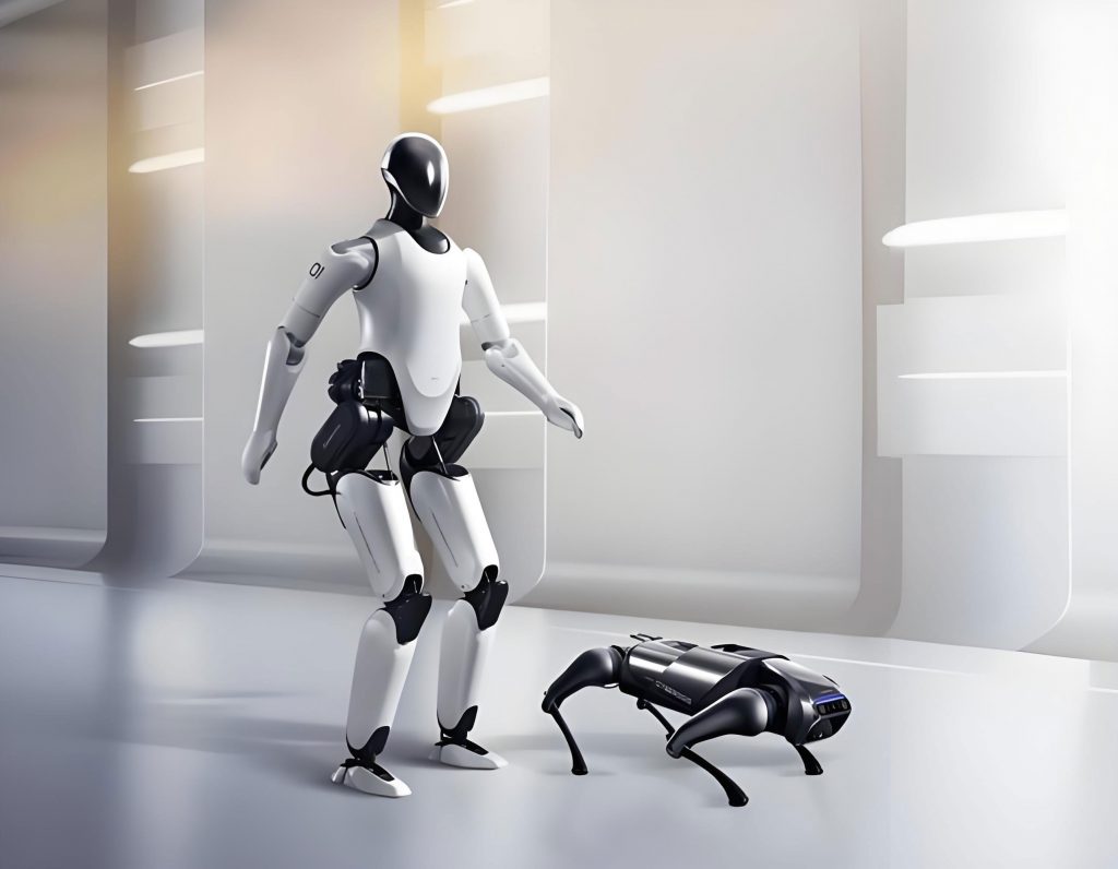
The pursuit of advanced bionic robot platforms capable of navigating complex, unstructured environments—such as planetary surfaces, disaster zones, or deep-sea terrains—has driven significant research into legged locomotion. Among various configurations, hexapod bionic robot designs offer an excellent compromise between static stability and mechanical complexity. This analysis focuses on a critical phase in the locomotion of such a bionic robot: its body motion during the support phase of a tripod gait. During this phase, with three legs firmly planted on the ground, the torso and the supporting legs constitute a parallel mechanism. Understanding the kinematic properties of this mechanism, specifically its Jacobian matrix, is paramount for tasks such as workspace analysis, dimensional synthesis, trajectory planning, and coordinated motion control of the entire bionic robot.
When walking with a stable tripod gait, a hexapod bionic robot alternates between two sets of three legs. While one set (e.g., the front-left, rear-left, and middle-right legs) is in contact with the ground providing support and propulsion, the other set swings forward. This configuration transforms the robot’s body into a 3-UrRS parallel mechanism. Here, ‘Ur’ denotes a composite universal joint formed by the coxa (roll) and femur (pitch) joints of a leg, ‘R’ represents the knee (pitch) joint, and ‘S’ models the point contact of the foot with the ground as a spherical joint. The schematic of this parallel mechanism, central to the bionic robot‘s propulsion, is shown below.
The kinematic analysis of this parallel mechanism, inherent to the bionic robot‘s walking strategy, can be elegantly performed using screw theory and the concept of reciprocal products. This approach offers a geometric and unified method to determine mobility and establish the Jacobian matrix without the need for first deriving explicit position solutions and then differentiating them—a process that can be cumbersome and prone to singularities.
Freedom and Constraint Analysis of the 3-UrRS Mechanism
A single leg of the hexapod bionic robot, when detached, possesses six degrees of freedom (DOF). The objective is to determine the collective mobility of the torso (the moving platform) when three such legs connect it to the fixed ground. Using the Grübler-Kutzbach criterion for spatial mechanisms:
$$ M = d(n – g – 1) + \sum_{i=1}^{g} f_i $$
For the 3-UrRS mechanism:
- Number of links, \( n = 8 \) (3 lower legs, 3 upper legs, 1 torso, 1 ground).
- Number of joints, \( g = 9 \) (3 Ur, 3 R, 3 S).
- Total joint freedom, \( \sum f_i = (3 \times 2) + (3 \times 1) + (3 \times 3) = 18 \).
- The mechanism has no common constraints (\(\lambda=0\)) and is spatial, so \( d = 6 \).
Substituting:
$$ M = 6(8 – 9 – 1) + 18 = 6 \times (-2) + 18 = 6 $$
This confirms the torso has 6 degrees of freedom relative to the ground, which is consistent with its ability to translate and rotate freely in space when the supporting feet are fixed. A more insightful approach uses screw theory. The kinematic chain of a single leg from the torso to the ground consists of six joints. Their screw coordinates \( \$_j \) (for \( j=1,…,6 \)) in a leg-fixed frame are:
$$
\begin{aligned}
\$_{1} &= (0, 1, 0;\ c_1, 0, -a_1) \quad \text{(Coxa Roll)} \\
\$_{2} &= (1, 0, 0;\ 0, -c_1, b_1) \quad \text{(Femur Pitch)} \\
\$_{3} &= (1, 0, 0;\ 0, -c_3, b_3) \quad \text{(Knee Pitch)} \\
\$_{4} &= (0, 0, 1;\ 0, 0, 0) \quad \text{(Foot Yaw)} \\
\$_{5} &= (0, 1, 0;\ 0, 0, 0) \quad \text{(Foot Roll)} \\
\$_{6} &= (1, 0, 0;\ 0, 0, 0) \quad \text{(Foot Pitch)}
\end{aligned}
$$
Finding the wrench (force or couple) that is reciprocal to all six joint screws of a leg identifies the constraint it applies to the torso. The reciprocal product is zero for all \( j \): \( \$^w \circ \$_j = 0 \). For this serial chain, no non-trivial wrench exists that is reciprocal to all six screws. This means an isolated leg imposes zero constraints on the torso’s motion; it is a 6-DOF serial chain itself. Therefore, three such legs connecting the torso to the ground do not overconstrain it, resulting in a 6-DOF parallel mechanism for the bionic robot body.
Jacobian Matrix Formulation via Screw Theory
The Jacobian matrix for a parallel mechanism relates the velocity of the moving platform (torso) to the actuated joint rates. For a bionic robot in a tripod stance, the actuators are typically located at the coxa, femur, or knee joints. We define the platform twist as \( \$_P = (\boldsymbol{\omega}_P^T, \boldsymbol{v}_P^T)^T \), where \( \boldsymbol{\omega}_P \) is the angular velocity and \( \boldsymbol{v}_P \) is the linear velocity of the platform centroid.
For the \( i\)-th leg (\( i=1,2,3 \)), the kinematic equation is:
$$ \$_P = \mathbf{J}_{s,i} \dot{\boldsymbol{\theta}}_i $$
where \( \mathbf{J}_{s,i} = [\$_{1,i}, \$_{2,i}, …, \$_{6,i}] \) is the \( 6 \times 6 \) Jacobian of the serial limb, and \( \dot{\boldsymbol{\theta}}_i = (\dot{\theta}_{1,i}, …, \dot{\theta}_{6,i})^T \).
The key to finding the parallel mechanism’s Jacobian is to identify the wrenches that the \( i\)-th leg can transmit to the platform when specific joints are actuated (locked). These transmission wrenches are reciprocal to all passive joint screws in that leg. By applying the reciprocal product between these transmission wrenches and the platform twist, we eliminate the passive joint rates.
Let \( \mathbf{J}_{r,i} \) be a matrix whose rows are the Plücker coordinates of the transmission wrenches for leg \( i \). Then,
$$ \mathbf{J}_{r,i} \$_P = \mathbf{J}_{\theta,i} \dot{\boldsymbol{q}}_i $$
where \( \dot{\boldsymbol{q}}_i \) is the vector of actuated joint rates for leg \( i \), and \( \mathbf{J}_{\theta,i} \) is a diagonal matrix with entries being the reciprocal products between the transmission wrenches and their corresponding actuated joint screws. Assembling for all three legs:
$$
\mathbf{J}_r \$_P = \mathbf{J}_{\theta} \dot{\boldsymbol{q}}
$$
where \( \mathbf{J}_r = [\mathbf{J}_{r,1}^T, \mathbf{J}_{r,2}^T, \mathbf{J}_{r,3}^T]^T \) is a \( 6 \times 6 \) matrix, \( \mathbf{J}_{\theta} \) is a \( 6 \times 6 \) diagonal matrix, and \( \dot{\boldsymbol{q}} = (\dot{\boldsymbol{q}}_1^T, \dot{\boldsymbol{q}}_2^T, \dot{\boldsymbol{q}}_3^T)^T \). The overall Jacobian matrix \( \mathbf{J} \) of the parallel mechanism, such that \( \$_P = \mathbf{J} \dot{\boldsymbol{q}} \), is then:
$$ \mathbf{J} = \mathbf{J}_r^{-1} \mathbf{J}_{\theta} $$
The specific form of \( \mathbf{J}_r \) and \( \mathbf{J}_{\theta} \) depends entirely on the choice of actuated joints in each leg of the bionic robot. We analyze three fundamental actuation schemes for a single leg.
Actuation Scheme 1: Coxa (Joint 1) and Knee (Joint 3) Actuated
When knee joint \( \$_{3,i} \) is locked, the passive joints are \( \$_{1,i}, \$_{2,i}, \$_{4,i}, \$_{5,i}, \$_{6,i} \). The wrench reciprocal to this system is a pure force passing through the foot contact point \( F_i \) and parallel to the knee/foot-pitch axis (\( \mathbf{s}_{6,i} \)): \( \$_{r1,i}^w = (\mathbf{s}_{6,i}; \mathbf{f}_i \times \mathbf{s}_{6,i}) \). When the coxa joint \( \$_{1,i} \) is locked, the passive joints are \( \$_{2,i}, \$_{3,i}, \$_{4,i}, \$_{5,i}, \$_{6,i} \). The reciprocal wrench is a force along the line connecting the coxa pivot \( D_i \) to the foot point \( F_i \): \( \$_{r3,i}^w = (\mathbf{f}_i – \mathbf{d}_i; \mathbf{f}_i \times (\mathbf{f}_i – \mathbf{d}_i)) \). Therefore:
$$
\mathbf{J}_{r,i} = \begin{bmatrix} (\mathbf{f}_i \times \mathbf{s}_{6,i})^T & \mathbf{s}_{6,i}^T \\ \mathbf{f}_i \times (\mathbf{f}_i – \mathbf{d}_i)^T & (\mathbf{f}_i – \mathbf{d}_i)^T \end{bmatrix}, \quad
\mathbf{J}_{\theta,i} = \begin{bmatrix} \$_{r1,i}^w \circ \$_{1,i} & 0 \\ 0 & \$_{r3,i}^w \circ \$_{3,i} \end{bmatrix}
$$
Actuation Scheme 2: Femur (Joint 2) and Knee (Joint 3) Actuated
With knee joint \( \$_{3,i} \) locked, the reciprocal wrench (found from the passive joints \( \$_{1,i}, \$_{2,i}, \$_{4,i}, \$_{5,i}, \$_{6,i} \)) is now a force along the line from the intersection point \( W_i \) of the femur and first foot-joint axes to the foot point \( F_i \): \( \$_{r2,i}^w = (\mathbf{e}_i – \mathbf{f}_i; \mathbf{e}_i \times (\mathbf{e}_i – \mathbf{f}_i)) \). With the femur joint \( \$_{2,i} \) locked, the reciprocal wrench is the same as \( \$_{r3,i}^w \) from Scheme 1.
$$
\mathbf{J}_{r,i} = \begin{bmatrix} \mathbf{e}_i \times (\mathbf{e}_i – \mathbf{f}_i)^T & (\mathbf{e}_i – \mathbf{f}_i)^T \\ \mathbf{f}_i \times (\mathbf{f}_i – \mathbf{d}_i)^T & (\mathbf{f}_i – \mathbf{d}_i)^T \end{bmatrix}, \quad
\mathbf{J}_{\theta,i} = \begin{bmatrix} \$_{r2,i}^w \circ \$_{2,i} & 0 \\ 0 & \$_{r3,i}^w \circ \$_{3,i} \end{bmatrix}
$$
Actuation Scheme 3: Coxa (Joint 1) and Femur (Joint 2) Actuated
With coxa joint \( \$_{1,i} \) locked, the reciprocal wrench is \( \$_{r2,i}^w \) from Scheme 2. With femur joint \( \$_{2,i} \) locked, the reciprocal wrench is \( \$_{r1,i}^w \) from Scheme 1.
$$
\mathbf{J}_{r,i} = \begin{bmatrix} \mathbf{e}_i \times (\mathbf{e}_i – \mathbf{f}_i)^T & (\mathbf{e}_i – \mathbf{f}_i)^T \\ \mathbf{f}_i \times \mathbf{s}_{6,i}^T & \mathbf{s}_{6,i}^T \end{bmatrix}, \quad
\mathbf{J}_{\theta,i} = \begin{bmatrix} \$_{r2,i}^w \circ \$_{2,i} & 0 \\ 0 & \$_{r1,i}^w \circ \$_{1,i} \end{bmatrix}
$$
The complete actuation strategy for the bionic robot‘s parallel mechanism can be any combination of these schemes across the three legs. The table below summarizes the transmission wrenches for all possible single-leg actuation pairs, which are the building blocks for the full parallel mechanism Jacobian.
| Actuated Joint Pair | Transmission Wrench 1 (Locking Joint A) | Transmission Wrench 2 (Locking Joint B) |
|---|---|---|
| Joint 1 & Joint 3 | Force through \( F_i \parallel \mathbf{s}_{6,i} \) (\( \$_{r1,i}^w \)) | Force along line \( D_i F_i \) (\( \$_{r3,i}^w \)) |
| Joint 2 & Joint 3 | Force along line \( W_i F_i \) (\( \$_{r2,i}^w \)) | Force along line \( D_i F_i \) (\( \$_{r3,i}^w \)) |
| Joint 1 & Joint 2 | Force along line \( W_i F_i \) (\( \$_{r2,i}^w \)) | Force through \( F_i \parallel \mathbf{s}_{6,i} \) (\( \$_{r1,i}^w \)) |
| Joint 1 & Joint 4/5/6 | Constraint depends on specific locked foot joint | Wrench reciprocal to other 5 joints |
For the common bionic robot design where the foot is not actuated, the practical actuation schemes involve only the coxa, femur, and knee joints (Joints 1, 2, 3). This gives \( 3^3 = 27 \) possible actuation combinations for the full parallel mechanism. The general form of the Jacobian for any combination is constructed by assembling the appropriate \( \mathbf{J}_{r,i} \) and \( \mathbf{J}_{\theta,i} \) blocks for each leg \( i \) according to its chosen actuation scheme.
Simulation and Validation
To verify the correctness of the Jacobian derived via screw theory for the bionic robot parallel mechanism, a kinematic simulation was performed. A model of the 3-UrRS mechanism was created, with Actuation Scheme 1 (Coxa and Knee actuated) used for all three legs. The actuated joints were assigned a constant angular velocity of \( 30^\circ/s \).
At a specific instant \( t = 1.02s \), the positions of all joint points (\( D_i, F_i \)) and the platform centroid were extracted from the simulation. The Plücker coordinates for the joint screws \( \$_{j,i} \) and the transmission wrenches \( \$_{r1,i}^w, \$_{r3,i}^w \) were computed. These were used to construct the instantaneous \( \mathbf{J}_r \) and \( \mathbf{J}_{\theta} \) matrices, yielding the overall Jacobian \( \mathbf{J} \):
$$
\mathbf{J} =
\begin{bmatrix}
-0.300 & -0.170 & 0.080 & -0.097 & 0.220 & -0.0021 \\
0.110 & -0.270 & -0.260 & 0.184 & 0.155 & 0.0001 \\
0.050 & 0.0014 & 0.410 & 0.016 & -0.670 & 0.0002 \\
-0.060 & 0.0040 & 0.0617 & -0.002 & 0.039 & 0 \\
-0.160 & -0.0080 & 0.0677 & 0.0006 & 0.073 & 0 \\
-0.0636 & 0.0148 & 0.0319 & 0.0064 & 0.030 & 0
\end{bmatrix}
$$
Using the known actuated joint velocity vector \( \dot{\boldsymbol{q}} \), the platform twist \( \$_P = \mathbf{J} \dot{\boldsymbol{q}} \) was calculated. The computed linear and angular velocity components showed exact agreement with the velocities of the platform centroid measured directly in the simulation at \( t=1.02s \), thereby validating the derived Jacobian matrix formulation.
Singularity Considerations for the Bionic Robot
The performance and control of the bionic robot are critically affected by singular configurations of its underlying parallel mechanism. Singularities occur when \( \mathbf{J}_r \) or \( \mathbf{J}_{\theta} \) becomes singular. Using the screw theory formulation, these can be interpreted geometrically:
- Inverse Kinematic Singularity: Occurs when \( \mathbf{J}_{\theta} \) is singular. This happens if a transmission wrench becomes reciprocal to its corresponding actuated joint screw (i.e., \( \$_{rK,i}^w \circ \$_{K,i} = 0 \)). For example, in Scheme 1, this occurs if the force along \( D_iF_i \) is perpendicular to the knee joint axis, a configuration typically at the boundary of the workspace.
- Forward Kinematic Singularity: Occurs when \( \mathbf{J}_r \) is singular. This is when the six transmission wrenches (two from each of the three legs) become linearly dependent. For a bionic robot stance, this could happen if the lines of action of all forces become coplanar or intersect in a degenerate manner, leading to an uncontrollable degree of freedom for the torso (e.g., a pure rotation about a vertical axis when all feet are collinear).
- Combined Singularity: Occurs when both conditions happen simultaneously.
The Jacobian derived via reciprocal screws provides clear insight into these conditions, allowing them to be avoided during the bionic robot‘s gait planning and controller design.
Conclusion
This analysis has demonstrated the application of screw theory and reciprocal products to model the tripod-support phase of a hexapod bionic robot as a 3-UrRS parallel mechanism. The method provides a powerful and geometrically intuitive framework for directly establishing the complete Jacobian matrix without resorting to derivative of complex positional equations. The analysis confirms the 6-DOF nature of the torso and derives the general form of the Jacobian for various leg actuation strategies, which is fundamental for the motion control of the bionic robot.
The resulting Jacobian matrix is crucial for subsequent research and development tasks essential for a functional bionic robot, including:
- Workspace Analysis: Mapping the reachable positions and orientations of the torso relative to the fixed feet.
- Kinematic Optimization: Performing dimensional synthesis to maximize dexterity, minimize actuator forces, or avoid singularities within the required workspace.
- Dynamics and Control: Formulating the equations of motion and designing advanced model-based controllers for stable and efficient locomotion.
- Trajectory Planning: Generating smooth and singularity-free body trajectories for the bionic robot during complex maneuvers.
Ultimately, a deep understanding of this core parallel mechanism’s kinematics significantly advances the design and control of robust, agile, and truly autonomous legged bionic robot systems.