
In recent years, the deployment of humanoid robots in unstructured environments such as emergency rescue, healthcare, and intelligent manufacturing has demanded significant advances in dynamic stability and environmental adaptability. The design of the ankle joint is a critical factor that determines the locomotion performance and terrain adaptability of a humanoid robot. Compared with traditional serial ankle mechanisms, parallel mechanisms offer higher stiffness, lower moving inertia, and better force transmission characteristics, which are beneficial for agile and robust dynamic motions. However, the kinematic complexity and strong coupling of parallel structures pose challenges for dynamic modeling and whole-body control. Moreover, conventional control algorithms rarely incorporate momentum coordination into the whole-body control architecture, limiting the balancing capability during highly dynamic tasks. To address these issues, this paper presents a systematic study on a novel two-degree-of-freedom (2-DOF) parallel ankle joint for humanoid robots, followed by a momentum coordination method based on the robot dynamics, and finally a hierarchical stability control framework that integrates the proposed momentum coordination strategy. The remainder of this article is organized as follows: Section 2 describes the mechanical design and kinematics of the parallel ankle joint; Section 3 develops the dynamic models and the momentum coordination method; Section 4 proposes the hierarchical control framework with model predictive control (MPC) and whole-body control (WBC), along with experimental validation; Section 5 concludes the paper.
1. Introduction and Motivation
Humanoid robots are designed to operate in human-centered environments, where they must perform complex locomotion tasks such as walking, running, climbing, and maintaining balance under external perturbations. The ankle joint plays an essential role in these tasks because it directly controls the foot–ground interaction and contributes to the overall stability of the robot. In many existing humanoid robots, the ankle joint is implemented as a serial mechanism with two or three rotational axes driven by motors mounted near the foot. Although such a design simplifies kinematic modeling, it inevitably increases the rotational inertia of the lower leg, reduces the dynamic response, and limits the ability to absorb impact forces during locomotion. In contrast, a parallel ankle joint can place the actuators closer to the knee or hip, thereby reducing the leg inertia and improving the force transmission efficiency. However, the closed-loop structure of a parallel mechanism introduces coupled motions and complex constraints that must be carefully addressed in both kinematics and dynamics.
From a control perspective, the stability of a humanoid robot during dynamic locomotion depends on the coordinated generation and regulation of whole-body momentum. Traditional position-based controllers, such as those relying solely on zero-moment point (ZMP) tracking, often treat the ankle joint as a position source and neglect the momentum distribution among the body segments. This can lead to poor disturbance rejection and limited mobility on uneven terrain. Recent advances in model predictive control and whole-body control have shown that integrating momentum regulation into a hierarchical control framework can significantly improve the robustness of legged robots. Nevertheless, the application of such methods to humanoid robots with parallel ankle joints remains relatively unexplored, especially when the parallel mechanism introduces additional dynamic coupling between the ankle joint and the rest of the body.
In this work, we aim to bridge this gap by combining mechanical design, dynamic modeling, and hierarchical control. We propose a novel 2-DOF parallel ankle joint that significantly reduces the leg inertia of a humanoid robot. We then derive a centroidal momentum coordination method that uses ankle torque information to generate a reference angular momentum trajectory, and we formulate a quadratic programming (QP) optimizer to harmonize momentum tasks with posture tasks. Finally, we embed the momentum coordination method into a layered control architecture consisting of an MPC for center-of-mass (COM) trajectory generation and a WBC for real-time joint torque computation. Extensive simulations and physical experiments on a humanoid robot platform demonstrate the effectiveness of the proposed methods.
2. Kinematic Analysis of the Parallel Ankle Joint
2.1 Structural Design and Degrees of Freedom
The proposed parallel ankle joint is depicted conceptually in the CAD model and kinematic schematic. The mechanism consists of two identical kinematic chains connecting the shank (lower leg) to the foot. Each chain comprises a rotating actuator, a connecting rod, and a spherical joint. A central universal joint at the ankle center connects the shank to the foot, providing the instantaneous center of rotation. The two actuators are mounted at the knee position with non-coaxial layouts, which effectively lowers the center of mass of the leg and reduces the rotational inertia. Furthermore, the large foot sole enables a stable support polygon in both the sagittal and frontal planes.
To verify the mobility of the mechanism, we employ the Kutzbach–Grübler formula:
$$ F = d(n – p – 1) + \sum_{i=1}^{p} f_i + v – \xi $$
where \(d=6\) is the order of the spatial mechanism, \(n=6\) is the number of links, \(p=7\) is the number of joints, \(f_i\) is the degree of freedom of the \(i\)-th joint, \(v\) is the redundancy correction, and \(\xi\) is the passive degree of freedom. Substituting the values gives \(F=2\), confirming that the mechanism has exactly two independent degrees of freedom. These correspond to ankle roll (inversion/eversion) and ankle pitch (dorsiflexion/plantarflexion), which are sufficient for stable bipedal locomotion.
2.2 Forward and Inverse Kinematics
Let the world frame be \(\mathcal{W}\) with its origin at the projection of the robot’s COM on the ground, the \(x\)-axis pointing forward, the \(y\)-axis pointing to the left, and the \(z\)-axis pointing upward. The ankle pose with respect to the world frame can be obtained by multiplying the homogeneous transformation matrices along the leg chain. For the left leg, the transformation from the torso frame to the ankle frame is:
$$ {}^{0}\mathbf{T}_{6} = {}^{0}\mathbf{T}_{1} {}^{1}\mathbf{T}_{2} {}^{2}\mathbf{T}_{3} {}^{3}\mathbf{T}_{4} {}^{4}\mathbf{T}_{5} {}^{5}\mathbf{T}_{6} $$
and similarly for the right leg. The inverse kinematics problem for the parallel ankle joint is to compute the actuator angles \(\boldsymbol{\theta} = [\theta_1, \theta_2]^T\) given the desired ankle orientation \(\mathbf{x}_a = [q_4, q_5]^T\), where \(q_4\) is the roll angle and \(q_5\) is the pitch angle. Based on the geometric relationships of the closed-loop chains, we derive:
$$ \theta_i = \arcsin \left( \frac{b^2 – c^2 + a^2 – \sqrt{b^2 c^2 – (b^2 + c^2 – a^2)^2}}{a^2 + b^2} \right) $$
where the intermediate variables \(a\), \(b\), and \(c\) are functions of the positions of points \(A_i\), \(B_i\), and \(C_i\) in the mechanism. The detailed derivation follows from the triangle identities in each limb.
2.3 Jacobian Matrix
To map the actuator velocities to the ankle angular velocities, we differentiate the loop-closure equations. Let \(\boldsymbol{\omega}\) be the angular velocity of the foot and \(\mathbf{v}\) the linear velocity of the ankle center. The velocity constraint for limb \(i\) is:
$$ \mathbf{r}_{rod_i} \cdot \mathbf{v} + \mathbf{r}_{rod_i} \cdot (\boldsymbol{\omega} \times \mathbf{r}_{bar_i}) = \dot{\theta}_i (\mathbf{r}_{rod_i} \times \mathbf{r}_{bar_i}) \cdot \mathbf{s}_{1_i} $$
Collecting both limbs yields:
$$ \mathbf{J}_x \dot{\mathbf{x}} = \mathbf{J}_{\theta} \dot{\boldsymbol{\theta}} $$
where \(\dot{\mathbf{x}} = [\mathbf{v}^T, \boldsymbol{\omega}^T]^T\) is the spatial velocity of the foot. The ankle Jacobian \(\mathbf{J}_a\) that relates the actuator velocities to the ankle roll and pitch rates is then:
$$ \dot{\boldsymbol{\theta}} = \mathbf{J}_a \dot{\mathbf{x}}_a $$
This Jacobian is essential for both kinematic control and singularity analysis. The mechanism is singular when \(\det(\mathbf{J}_a)=0\), which occurs at the boundary of the workspace. In practice, the designed workspace of the ankle is \([-40^\circ, 40^\circ]\) for roll and \([-40^\circ, 20^\circ]\) for pitch, far away from singular configurations.
2.4 Experimental Validation of Kinematics
We implemented the proposed parallel ankle joint on a physical humanoid robot platform. The robot has a total mass of 45 kg and a height of 1.6 m. Each leg has six actuated joints: three at the hip, one at the knee, and two at the ankle using the parallel mechanism. The actuator stroke is \([-70^\circ, 50^\circ]\), which covers the required ankle workspace. We conducted squatting, stepping, and omnidirectional walking experiments. The measured joint angles and actuator positions showed consistent periodic patterns, as summarized in Table 1.
| Parameter | Value | Unit |
|---|---|---|
| Degrees of freedom | 2 | – |
| Roll range | [-40, 40] | deg |
| Pitch range | [-40, 20] | deg |
| Actuator stroke | [-70, 50] | deg |
| Link length (upper bar) | 89 | mm |
| Link length (lower bar) | 89 | mm |
| Connecting rod 1 | 250 | mm |
| Connecting rod 2 | 187 | mm |
| Mass of optimized lower leg | 2.8 | kg |
The experimental results confirmed that the parallel ankle joint enables smooth and stable motions in squatting, stepping, and walking. The two actuator angles differ by a constant offset at the initial configuration due to the non-coaxial mounting, which is fully accounted for in the inverse kinematics. The lightweight design reduced the lower leg mass from 5.9 kg to 2.8 kg, a reduction of more than 50%, significantly improving the dynamic response of the leg.
3. Momentum Coordination Method Based on the Humanoid Robot Dynamics
3.1 Dynamic Models
To design a model-based momentum controller, we first establish a floating-base dynamic model. The generalized coordinates are partitioned into the floating base (torso pose) and the joint coordinates:
$$ \mathbf{q} = [\mathbf{q}_{fb}^T, \mathbf{q}_j^T]^T $$
The equations of motion can be written as:
$$ \mathbf{M}(\mathbf{q}) \begin{bmatrix} \dot{\mathbf{v}}_c \\ \ddot{\mathbf{q}} \end{bmatrix} + \mathbf{C}(\mathbf{q}, \dot{\mathbf{q}}) = \begin{bmatrix} \mathbf{0} \\ \boldsymbol{\tau} \end{bmatrix} + \begin{bmatrix} \mathbf{J}_c^T \boldsymbol{\lambda} \\ \mathbf{J}_j^T \boldsymbol{\lambda} \end{bmatrix} $$
where \(\mathbf{M}\) is the inertia matrix, \(\mathbf{C}\) accounts for Coriolis, centrifugal, and gravitational effects, \(\boldsymbol{\tau}\) is the joint torque vector, \(\boldsymbol{\lambda}\) is the contact wrench, and \(\mathbf{J}_c\), \(\mathbf{J}_j\) are the corresponding Jacobians. The dynamic model incorporates the parallel ankle joint mass and inertia properties through the inertia matrix \(\mathbf{M}\). Since the actuators are relocated to the knee, the leg inertia is substantially reduced, which simplifies the dynamic coupling between the ankle and the hip.
For the purpose of centroidal momentum control, we also adopt a single rigid body centroidal model. Let \(\mathbf{p}_{com} \in \mathbb{R}^3\) be the center of mass position, \(\mathbf{l}_c \in \mathbb{R}^3\) the centroidal angular momentum, \(\mathbf{p}_{zmp}\) the zero moment point, and \(\mathbf{f}_{ext}\) the external ground reaction force. The equations governing the COM and angular momentum are:
$$ m \ddot{\mathbf{p}}_{com} = m \mathbf{g} + \mathbf{f}_{ext} $$
$$ \dot{\mathbf{l}}_c = (\mathbf{p}_{zmp} – \mathbf{p}_{com}) \times \mathbf{f}_{ext} $$
These equations provide a compact representation of the interaction between the robot’s momentum and the external contact forces, which is essential for the momentum coordination strategy.
3.2 Ankle Torque Computation
We propose a three-stage momentum coordination framework: (1) compute the required ankle torques from the dynamic model; (2) generate a reference centroidal angular momentum based on the ankle torque deficit; (3) solve a quadratic program to optimize the whole-body motion while respecting task constraints.
Using the floating-base dynamics, we define a desired closed-loop impedance behavior for the COM and the torso orientation. The virtual contact wrench at the foot is decomposed into a hip part and an ankle part:
$$ \boldsymbol{\tau}_v^{hip} + \boldsymbol{\tau}_v^{ankle} = \mathbf{A}_d^{-T} (\mathbf{w}_c^{ff} + \mathbf{w}_c^{imp} – \mathbf{w}_g) $$
where \(\mathbf{w}_c^{ff}\) is the feedforward wrench computed from the desired COM trajectory, \(\mathbf{w}_c^{imp}\) is the feedback impedance wrench, and \(\mathbf{w}_g\) is the gravity wrench. The ankle torque is the component that directly acts on the parallel ankle mechanism. When the norm of the ankle torque exceeds a predefined threshold \(\boldsymbol{\tau}_v^{th}\), the robot detects that the ankle alone is insufficient to maintain balance and needs to mobilize the whole-body momentum.
3.3 Centroidal Angular Momentum Generation
The reference rate of change of the centroidal angular momentum is generated from the excess ankle torque:
$$ \dot{\mathbf{l}}_c^{ref} = \boldsymbol{\tau}_v^{ankle} – \boldsymbol{\tau}_v^{th} $$
Integrating this equation over time yields the desired centroidal angular momentum reference \(\mathbf{l}_c^{ref}\). This reference is then used as an input to a QP-based motion optimizer. The angular momentum of the humanoid robot can be expressed as:
$$ \mathbf{l}_c = \bar{\mathbf{A}} \dot{\mathbf{q}} $$
where \(\bar{\mathbf{A}}\) is the centroidal momentum matrix. We split the whole-body velocity into an optimized part \(\dot{\mathbf{x}}_a\) and a fixed part \(\dot{\mathbf{x}}_u\). The QP is formulated as:
$$ \min_{\dot{\mathbf{x}}_a} \ \frac{1}{2} \boldsymbol{\delta}_m^T \mathbf{Q}_m \boldsymbol{\delta}_m + \frac{1}{2} \boldsymbol{\delta}_n^T \mathbf{Q}_n \boldsymbol{\delta}_n $$
subject to
$$ \mathbf{A}_a \dot{\mathbf{x}}_a + \mathbf{A}_u \dot{\mathbf{x}}_u = \mathbf{l}_c^{ref} + \boldsymbol{\delta}_m $$
$$ \dot{\mathbf{x}}_a^{des} – \dot{\mathbf{x}}_a = \boldsymbol{\delta}_n $$
$$ \dot{\mathbf{x}}_a^{min} \leq \dot{\mathbf{x}}_a \leq \dot{\mathbf{x}}_a^{max} $$
Here \(\boldsymbol{\delta}_m\) and \(\boldsymbol{\delta}_n\) are slack variables that allow for soft task priorities, \(\mathbf{Q}_m\) and \(\mathbf{Q}_n\) are positive definite weighting matrices. The optimizer trades off between tracking the desired momentum and maintaining a natural posture reference, while respecting joint velocity and position limits. This formulation effectively coordinates the whole-body momentum distribution and prevents the robot from adopting awkward postures during dynamic maneuvers.
3.4 Simulation Results of Momentum Coordination
We validated the momentum coordination method in a high-fidelity simulation environment (Drake). The humanoid robot model with the parallel ankle joint was commanded to perform stepping and forward walking. We recorded the ankle forces and torques, the centroidal angular momentum, and the COM trajectory. Figure 1 shows the humanoid robot model used in the simulation and the experimental validation.
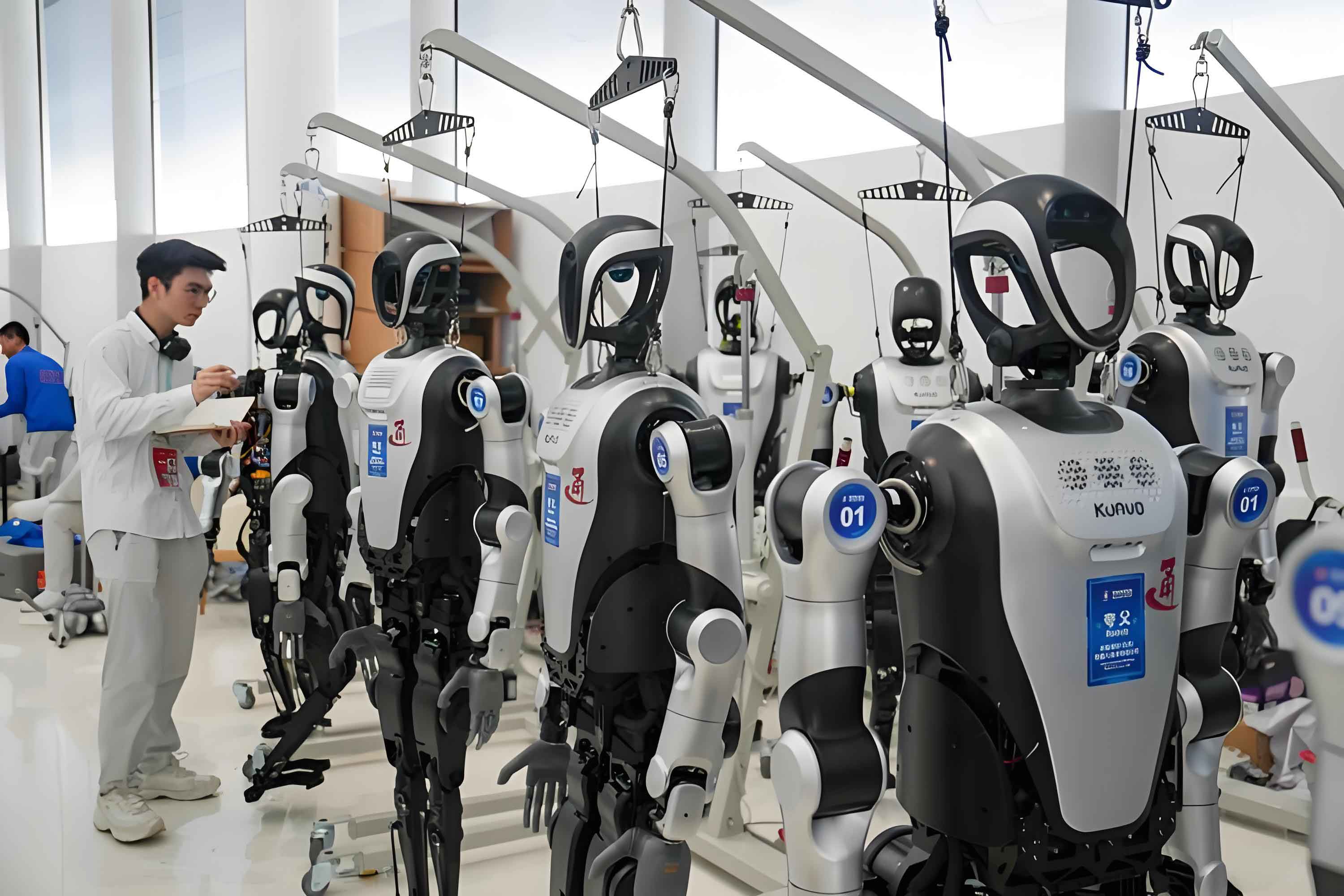
During the stepping motion, the ankle forces and torques exhibited clear periodic patterns. The vertical force at the ankle reached approximately 381 N, while the horizontal forces remained below 53 N. The ankle torque around the pitch axis oscillated between \(-7.33\) and \(7.30\) N·m. When the robot transitioned to forward walking, the horizontal ankle forces changed slightly, but the vertical force remained essentially the same. The reference centroidal angular momentum around the yaw axis was computed from the ankle torque using the proposed method. In both simulation and physical experiments, the angular momentum showed a periodic and bounded pattern, confirming that the momentum coordination method effectively converts ankle torque information into a meaningful whole-body momentum reference.
Figure 2 compares the COM trajectory with and without the momentum coordination method during forward walking. Without momentum coordination, the COM trajectory showed noticeable oscillations in the lateral direction. With the proposed method, the COM trajectory became significantly smoother, and the lateral deviation was reduced, demonstrating that the momentum coordination suppresses disturbances from foot–ground contact and enhances dynamic balance.
4. Hierarchical Stability Control with Momentum Coordination
4.1 Overall Control Framework
The proposed stability control framework adopts a hierarchical architecture that combines model predictive control (MPC) for trajectory generation and whole-body control (WBC) for real-time torque computation. The overall structure is illustrated in the block diagram of our control system. At the top level, an MPC based on the linear inverted pendulum model (LIPM) receives the desired forward velocity and generates a sequence of foothold positions and COM reference trajectories over a finite horizon. At the middle level, the momentum coordination method computes the desired centroidal angular momentum and adjusts the whole-body motion plan to ensure that the robot can track the MPC outputs without violating dynamic constraints. At the bottom level, a WBC formulates a quadratic program to compute joint torques that satisfy the desired task accelerations, contact constraints, and actuator limits.
4.2 ZMP Stability Criterion
The zero moment point (ZMP) is a fundamental metric for bipedal stability. It is defined as the point on the ground where the net moment of the ground reaction forces has zero horizontal components. For a humanoid robot in contact with the ground, the ZMP must lie inside the convex hull of the foot support polygon to ensure stability. The ZMP can be computed from the ground reaction force distribution:
$$ p_x = \frac{\int_S x \, \rho(\xi,\eta) \, dS}{\int_S \rho(\xi,\eta) \, dS}, \qquad p_y = \frac{\int_S y \, \rho(\xi,\eta) \, dS}{\int_S \rho(\xi,\eta) \, dS} $$
where \(\rho(\xi,\eta)\) is the vertical pressure distribution over the foot sole. In practice, we measure the ZMP using six-axis force/torque sensors mounted under the feet. The control objective is to keep the actual ZMP close to the reference ZMP while ensuring that the reference ZMP stays inside the support polygon.
4.3 Linear Inverted Pendulum Model and MPC
The LIPM simplifies the robot dynamics by assuming that the COM moves on a horizontal plane with constant height \(z_{com}\). Under this assumption, the horizontal COM dynamics are decoupled:
$$ \ddot{x}_{com} = \omega^2 (x_{com} – p_x) $$
$$ \ddot{y}_{com} = \omega^2 (y_{com} – p_y) $$
where \(\omega = \sqrt{g / z_{com}}\). We discretize these equations with a sampling period \(T_s\) to obtain a linear state-space model for prediction. The MPC optimizer solves the following quadratic program at each control step:
$$ \min_{\mathbf{p}_x, \mathbf{p}_y} \sum_{i=1}^{N} \left[ Q_x (\dot{x}_{com,i} – \dot{x}_{com,i}^d)^2 + R_x (p_{x,i} – p_{x,i}^{ref})^2 \right] + \sum_{i=1}^{N} \left[ Q_y (\dot{y}_{com,i} – \dot{y}_{com,i}^d)^2 + R_y (p_{y,i} – p_{y,i}^{ref} – y_s)^2 \right] $$
subject to the LIPM dynamics and the foothold reachability constraints. The solution provides the optimal ZMP positions and the corresponding COM trajectories for the next \(N\) steps. This approach allows the robot to react to external pushes and track a desired walking velocity while respecting the ZMP constraints.
4.4 Whole-Body Control with Friction Cone Constraints
The WBC computes joint torques from the desired task accelerations. The optimization variables include joint accelerations \(\ddot{\mathbf{q}}\), joint torques \(\boldsymbol{\tau}\), and contact wrenches \(\boldsymbol{\lambda}\). The QP formulation is:
$$ \min_{\ddot{\mathbf{q}}, \boldsymbol{\tau}, \boldsymbol{\lambda}} \sum_{i} \beta_i \| \mathbf{J}_i \ddot{\mathbf{q}} + \dot{\mathbf{J}}_i \dot{\mathbf{q}} – \mathbf{a}_i^{des} \|^2 $$
subject to the floating-base dynamics:
$$ \mathbf{M} \ddot{\mathbf{q}} + \mathbf{C} = \boldsymbol{\tau} + \mathbf{J}_c^T \boldsymbol{\lambda} $$
and the contact constraints for each foot:
$$ \mathbf{J}_{c,i} \ddot{\mathbf{q}} + \dot{\mathbf{J}}_{c,i} \dot{\mathbf{q}} = \mathbf{0} $$
In addition, the contact forces must satisfy friction cone constraints to avoid slipping. Since a full friction cone is nonlinear, we approximate it by a polyhedral cone as depicted conceptually in Figure 3. The linearized constraints are:
$$ |F_{x,i}| \leq \mu F_{z,i}, \quad |F_{y,i}| \leq \mu F_{z,i}, \quad F_{z,i} \geq 0 $$
where \(\mu\) is the friction coefficient. For the parallel ankle joint, the contact point is effectively the center of the foot sole, which is larger than that of a conventional serial ankle, providing a larger stability margin. The WBC solves the QP at a frequency of 1 kHz, producing joint torques that are sent directly to the motor drives.
4.5 State Estimation with Extended Kalman Filter
To provide accurate feedback to the controller, we implemented a state estimator based on the extended Kalman filter (EKF). The estimator fuses data from an inertial measurement unit (IMU), joint encoders, and foot force sensors. The state vector includes the torso pose, linear velocity, angular velocity, and the joint positions and velocities. The process model is derived from the floating-base dynamics, while the measurement model maps the state to the sensor outputs. The EKF recursively computes the optimal state estimate by minimizing the mean squared error. This estimator is robust to the switching contact conditions during walking, ensuring that the controller receives reliable state information in real time.
4.6 Balance Constraints
In addition to the ZMP constraint, we enforce several other balance constraints in the control framework:
- Friction constraint: The ground reaction forces must lie within the friction cone to prevent foot slipping.
- Joint limit constraint: Joint angles and velocities are bounded to avoid kinematic singularities and physical damage.
- Non-singular posture constraint: The knee joint angle is kept above a minimum value to ensure that the leg Jacobian remains full rank:
$$ L_{leg}^{real} \geq \lambda L_{leg} $$
where \(\lambda \in (0,1)\) is a safety factor. This constraint prevents the knee from hyper-extending and losing controllability.
5. Experimental Evaluation
5.1 Experimental Setup
The proposed control framework was implemented on a physical humanoid robot with the parallel ankle joint. The robot has a height of 1.6 m and a total mass of 45 kg. Each leg contains six drive units: three at the hip, one at the knee, and two actuators for the parallel ankle. The knee and ankle actuators use linkage transmissions, while the hip joints are directly driven. The robot communicates over an EtherCAT bus with a control cycle of 1 ms. In the experiments, the robot walked on a flat ground surface at a steady speed. The reference COM velocity was set to 0.4 m/s.
5.2 Walking Experiments and Motor Torque Analysis
During the walking experiments, we recorded the joint torques of all six motors on the left leg. Figure 4 shows the motor torque profiles from the simulation, and Figure 5 shows the corresponding physical measurements. The torque profiles of the hip roll, hip yaw, hip pitch, knee pitch, and the two ankle motors are presented in separate subplots. We observe the following characteristics:
| Joint | Range (N·m) | Pattern |
|---|---|---|
| Hip roll | [0, 31] | Periodic, small amplitude |
| Hip yaw | [-1, 10] | Quasi-periodic, small |
| Hip pitch | [-40, 50] | Continuous alternating drive/brake |
| Knee pitch | [-57, 20] | Large peak at touch-down |
| Ankle motor 1 | [-25, 30] | Complementary with motor 2 |
| Ankle motor 2 | [-30, 25] | Complementary with motor 1 |
The hip roll torque changes periodically to regulate lateral balance. The hip yaw torque remains small during straight walking, indicating that the robot maintains its heading direction without excessive corrective action. The hip pitch torque exhibits a typical “push-off” pattern: a positive peak during the late stance phase to propel the body forward, followed by a negative phase to decelerate the leg during the swing. The knee torque reaches its maximum magnitude at the moment of foot touchdown, which demonstrates the active compliance of the knee joint to absorb impact energy and reduce the vertical momentum spike. The two ankle motor torques are complementary in a way that reflects the parallel mechanism’s coupling: when one motor produces a positive torque, the other produces a negative torque to generate the desired ankle roll or pitch moment. This complementary behavior is a direct consequence of the parallel arrangement and is crucial for maintaining the foot in full contact with the ground.
5.3 ZMP Tracking Results
Figure 6 compares the reference ZMP and the measured ZMP during forward walking. In both the \(x\) and \(y\) directions, the measured ZMP closely tracks the reference, with a small cumulative error that grows over time due to integration drift and imperfect ground conditions. The maximum lateral deviation remains within 2 cm, which is well inside the support polygon of the foot. The experimental results confirm that the proposed hierarchical control framework with momentum coordination is able to maintain dynamic balance even when the robot is subjected to internal model errors and external disturbances.
5.4 Discussion
The experimental outcomes demonstrate that the integration of a parallel ankle joint with a momentum-coordinated hierarchical controller yields superior stability and adaptability for a humanoid robot. The reduced leg inertia allows faster joint torque responses, while the momentum coordination provides an additional layer of balance recovery that is not present in conventional ZMP tracking controllers. The MPC–WBC architecture handles the multi-objective optimization effectively, and the EKF ensures that the controller receives accurate state estimates despite the complex contact dynamics.
One limitation of the current study is that the experiments were conducted only on flat ground. Future work will extend the method to uneven terrain and push recovery scenarios. Moreover, the parallel ankle joint has a limited workspace in comparison to some serial designs; however, for most bipedal locomotion tasks, the achieved range is sufficient.
6. Conclusion
This paper presented a complete framework for the motion analysis and stability control of a humanoid robot equipped with a novel parallel ankle joint. We first designed a lightweight two-degree-of-freedom parallel ankle mechanism, validated its kinematics, and demonstrated its advantages in reducing leg inertia. We then developed a momentum coordination method based on the floating-base dynamic model and the centroidal angular momentum equation. The method computes ankle torques, generates a reference angular momentum, and uses a quadratic program to optimize the whole-body motion. Finally, we embedded this momentum coordination into a hierarchical control framework consisting of a linear inverted pendulum MPC and a whole-body controller. The WBC explicitly considers ZMP constraints, friction cone constraints, and joint limits. Simulations and physical experiments on a 45 kg humanoid robot confirmed that the proposed control framework achieves stable walking with smooth COM trajectories and reliable ZMP tracking. The results highlight the importance of co-designing the mechanical structure and the control algorithm for humanoid robots and open new possibilities for high-dynamic locomotion in complex environments.
In future work, we will extend the momentum coordination method to handle multiple contact modes, such as hand–foot contacts during climbing or crawling. We will also investigate the use of reinforcement learning to adapt the momentum reference generator online, thereby improving the robot’s ability to handle unforeseen disturbances. With the rapid advancement of actuators and sensors, we believe that the combination of parallel mechanisms and momentum-based hierarchical control will play a key role in the next generation of humanoid robots.