
In this thesis, I present my research on the whole-body motion control system for a wheeled humanoid robot that I developed in my laboratory. The robot integrates the dexterous manipulation of a dual-arm system with the mobility of a differential-drive base, and it is designed for indoor logistics, home service, and flexible manufacturing environments. One of the main challenges I faced is that the robot has more than 30 active degrees of freedom, which leads to strong kinematic coupling and high computational complexity. Conventional decoupled control approaches — where the mobile base first moves to a fixed position and then the arm executes a pick-and-place task — are inefficient and often fail to exploit the full capability of a humanoid robot. Therefore, I focused on whole-body motion control methods that coordinate all joints and the mobile base simultaneously in a single optimization framework.
My research covers the complete design cycle: mechanical structure, hardware architecture, low-level drivers, software integration, kinematic modeling, and two advanced control strategies. The first control strategy is based on quadratic programming (QP) with control barrier functions (CBF) for reactive whole-body manipulation. The second strategy is based on sequential linear-quadratic model predictive control (SLQ-MPC), which allows real-time constrained optimal control of the entire humanoid robot. I validated both methods through extensive simulations and physical experiments. The results show that the SLQ-MPC based method achieves a 96% success rate in random reach-and-pose tasks, while guaranteeing joint limits, velocity limits, self-collision avoidance, and tip-over prevention.
1. Introduction and Motivation
The development of humanoid robots has attracted significant attention due to the aging population and the increasing demand for automation in non-structured environments. A wheeled humanoid robot combines the dexterous manipulation capabilities of traditional robotic arms with the mobility of automated guided vehicles (AGVs), making it a promising platform for various applications such as medical care, home assistance, and industrial logistics. Unlike bipedal humanoid robots that require complex dynamic balancing, wheeled humanoid robots have a stable base, which simplifies the balance control and increases the payload capacity.
However, the high number of degrees of freedom and the strong coupling between the mobile base, legs, torso, arms, and hands make the motion control problem challenging. Traditional decoupled methods treat the mobile base and the arm separately: first, the base navigates to a goal pose, then the arm performs the manipulation task while the base is locked. This strategy is simple but slow and does not fully utilize the kinematic redundancy of the humanoid robot. To improve efficiency, I developed whole-body motion control algorithms that simultaneously use the base, legs, torso, and arm to achieve a desired end-effector pose while satisfying all physical constraints.
The main contributions of my research are as follows:
- Design and implementation of a complete hardware and software control system for a self-developed wheeled humanoid robot.
- Development of a whole-body kinematic model and a task-Jacobian based inverse kinematics solver.
- Formulation of a CBF-QP based reactive whole-body controller that handles joint position/velocity limits and self-collision avoidance.
- Development of an SLQ-MPC based whole-body motion controller that includes joint limits, control input bounds, collision avoidance, and tip-over prevention in a unified optimal control framework.
2. Hardware System Design of the Wheeled Humanoid Robot
2.1 Performance Specifications and Mechanical Structure
I designed the wheeled humanoid robot based on the target applications in indoor environments. The main performance indicators are listed in the following table.
| Parameter | Value |
|---|---|
| Height | 1700 mm |
| Weight | 80 kg |
| Protection rating | IP21 (indoor) |
| Active DOF | 32 |
| Maximum moving speed | 2 m/s |
| Single arm DOF | 6 |
| Arm reach | 600 mm |
| Arm payload | ≥3 kg (single), ≥6 kg (dual) |
| Hand DOF | 6 each |
| AI computing power | ≥100 TOPS |
| Battery | 48 V, 60 Ah |
| Endurance | ≥4 h |
The mechanical structure includes a two-wheel differential drive base, two driven wheels at the front, two caster wheels at the rear, three revolute joints per leg, one revolute joint in the torso, two revolute joints in the neck, and two 6-DOF arms with dexterous hands. The distribution of active degrees of freedom is summarized below.
| Part | Number of Joints |
|---|---|
| Mobile base | 2 (wheel velocities) |
| Legs | 3 |
| Torso | 1 |
| Head | 2 |
| Arms | 6×2 |
| Hands | 6×2 |
| Total | 32 |
2.2 Kinematic Modeling
I modeled the differential drive base first. Let \( \theta \) be the heading angle of the base, \( r \) the wheel radius, \( b \) the distance between the two driven wheels, and \( \omega_L, \omega_R \) the left and right wheel angular velocities. The base velocity in the world frame is given by:
$$
\begin{bmatrix} \dot{x} \\ \dot{y} \\ \dot{\theta} \end{bmatrix}
=
\begin{bmatrix}
\frac{r\cos\theta}{2} & \frac{r\cos\theta}{2} \\
\frac{r\sin\theta}{2} & \frac{r\sin\theta}{2} \\
\frac{r}{b} & -\frac{r}{b}
\end{bmatrix}
\begin{bmatrix} \omega_R \\ \omega_L \end{bmatrix}.
$$
For the 6-DOF arm, I used the Denavit–Hartenberg (D-H) convention. The forward kinematics of the arm is expressed as:
$$
T_{\text{arm}}(\mathbf q_{\text{arm}}) = T_1^0(q_1) T_2^1(q_2) \cdots T_6^5(q_6)
$$
where \( \mathbf q_{\text{arm}} \) is the vector of six joint angles. The D-H parameters of the right arm are shown in the following table.
| Joint \(i\) | \( \theta_i \) | \( d_i \) (m) | \( a_i \) (m) | \( \alpha_i \) |
|---|---|---|---|---|
| 1 | \( q_{\text{shoulder y}} \) | 0 | 0.15 | 0 |
| 2 | \( q_{\text{shoulder x}} + \pi/2 \) | 0.2 | 0.04 | \(-\pi/2\) |
| 3 | \( q_{\text{elbow z}} – \pi/2 \) | 0 | 0.15 | \( \pi/2 \) |
| 4 | \( q_{\text{elbow y}} – \pi/2 \) | 0 | 0.15 | \( \pi/2 \) |
| 5 | \( q_{\text{wrist x}} + \pi/2 \) | 0 | 0.12 | \( \pi/2 \) |
| 6 | \( q_{\text{wrist z}} \) | 0 | 0.1 | 0 |
Combining the base kinematics and the serial-chain kinematics of the legs, torso, and arm, I obtained the whole-body forward kinematics. By differentiating the forward kinematics, I derived the whole-body geometric Jacobian \( \mathbf J(\mathbf q) \) that maps the generalized velocity vector to the end-effector spatial velocity:
$$
\mathbf v_e =
\mathbf J(\mathbf q)
\begin{bmatrix} \mathbf u_{\text{base}} \\ \dot{\mathbf q}_s \end{bmatrix}
$$
where \( \mathbf u_{\text{base}} = [v_{\text{base}},\ \omega_{\text{base}}]^T \) is the base velocity and \( \mathbf q_s \) collects the leg, torso, and arm joint positions.
2.3 Hardware Architecture
I adopted a dual-controller architecture to provide sufficient computational resources for both real-time motion planning and AI-based perception. The two main controllers are a Raspberry Pi 5 and an NVIDIA Jetson Orin Nano. The Raspberry Pi 5 handles the upper body — the two arms and the torso — via its CAN expansion boards. The Jetson Orin Nano controls the legs and the base through its onboard CAN interface, and also processes the LiDAR, depth camera, and IMU data. The two controllers communicate via Ethernet using the DDS middleware of ROS2. The electrical design includes a 48 V lithium battery that powers the joint motors directly, while buck converters provide 24 V for the hands and head, and 19 V/5 V for the computers and sensors.
3. Software System Design
I built the robot software system on top of ROS2 (Humble distribution) using a layered and modular architecture. The overall software stack consists of three layers: the hardware driver layer, the middle control layer, and the top application layer. The middle layer includes state estimation, kinematics, local planning, and whole-body controllers. The top layer includes perception, navigation, and teleoperation modules.
3.1 Hardware Drivers with ros2_control
For the low-level joint control, I used the ros2_control framework combined with the ros2_canopen package. The CANopen master and device drivers are configured via YAML/BIN/DCF files, providing standardized interfaces for position, velocity, and torque feedback. Each joint motor is exposed to the ROS2 ecosystem through these interfaces. I configured the base wheels with velocity interfaces, the arm and leg joints with position/velocity/torque interfaces, and the IMU as a sensor component. The ros2_control resource manager loads the hardware components, while the controller manager provides joint trajectory controllers, joint state broadcasters, and velocity controllers. I also integrated the Gazebo simulator using the gz_ros2_control plugin for hardware-in-the-loop tests.
3.2 Motion Planning with MoveIt2
For upper-body motion planning, I integrated MoveIt2. I defined five planning groups: head, torso, left arm, right arm, and legs. The OMPL planner is used for arm planning, while a custom inverse kinematics solver handles the whole-body Jacobian. MoveIt2 also performs planning-scene management, collision checking, and trajectory smoothing. The moveit_servo package is used for real-time teleoperation of the end effector and individual joints.
3.3 Navigation with Nav2
For the mobile base, I used the Nav2 navigation framework. The robot receives a goal pose, and Nav2’s global planner computes a path using the map from the LiDAR while the local controller (DWB) follows the path in real time. The navigation stack communicates with the whole-body controller, allowing the base to move while the arm is performing a manipulation task.
3.4 Teleoperation and Autonomous Docking
I designed a teleoperation system using an Xbox wireless controller. The joystick commands are converted into either joint-space velocity commands (via JointJog) or Cartesian velocity commands (via TwistStamped) and then executed by the servo controller. For autonomous docking and charging, I used the opennav_docking package together with the isaac_ros_apriltag detector. A charging station is equipped with an Apriltag marker. The robot first navigates to a pre-pose, then uses the camera to detect the marker and performs closed-loop alignment until contact with the charging dock is established.
4. Whole-Body Motion Control Based on Quadratic Programming
4.1 Task Jacobian and Pseudoinverse
In this chapter, I consider a task to move the end effector to a desired pose \( \mathbf T_{\text{target}} \in SE(3) \). The residual in the Lie group sense is defined as:
$$
\mathbf e(\mathbf q) = \log\left( \mathbf T_{\text{target}}^{-1} \mathbf T_{\text{ee}}(\mathbf q) \right)^\vee \in \mathbb{R}^6,
$$
where \( \log(\cdot) \) is the logarithmic map from \( SE(3) \) to its Lie algebra, and \( (\cdot)^\vee \) converts a twist to a 6D vector. The task Jacobian \( \mathbf J_t(\mathbf q) \) is then defined as:
$$
\mathbf J_t(\mathbf q) = \frac{\partial \mathbf e}{\partial \mathbf q}.
$$
For a single task, the pseudoinverse solution is:
$$
\dot{\mathbf q} = – \alpha \mathbf J_t^{\dagger}(\mathbf q) \mathbf e(\mathbf q),
$$
where \( \alpha > 0 \) is the task gain. When multiple tasks are present, I can stack them with weights \( w_i \):
$$
\dot{\mathbf q} = \mathbf J_p^{\dagger} \mathbf v_p + \left( \mathbf I – \mathbf J_p^{\dagger} \mathbf J_p \right) \mathbf z,
$$
where \( \mathbf J_p \) is the primary task Jacobian and \( \mathbf z \) is the secondary task velocity projected into the null space.
I implemented this pseudoinverse controller using the Pinocchio library. However, experiments showed that this method often violates joint velocity limits or produces self-collisions, because it does not explicitly account for physical constraints. The success rate in random reach tasks was only 26%, confirming the need for a more constrained formulation.
4.2 QP-Based Whole-Body Control
I formulated the whole-body inverse kinematics as a quadratic program (QP). The decision variable is the joint velocity \( \dot{\mathbf q} \). The cost function is:
$$
\min_{\dot{\mathbf q}} \sum_i w_i \left\| \mathbf J_i \dot{\mathbf q} – K_i \mathbf v_i \right\|^2 + \gamma \| \dot{\mathbf q} \|^2,
$$
subject to:
$$
\underline{\mathbf q} \le \mathbf q \le \overline{\mathbf q}, \qquad \underline{\dot{\mathbf q}} \le \dot{\mathbf q} \le \overline{\dot{\mathbf q}},
$$
and the acceleration constraints:
$$
\underline{\mathbf a} \le \frac{\dot{\mathbf q}(t+\Delta t) – \dot{\mathbf q}(t)}{\Delta t} \le \overline{\mathbf a}.
$$
I wrote the QP in the standard form:
$$
\min_{\mathbf x} \frac{1}{2} \mathbf x^T \mathbf H \mathbf x + \mathbf h^T \mathbf x \quad \text{s.t. } \mathbf A \mathbf x \le \mathbf b,
$$
where \( \mathbf x \) is the decision vector, \( \mathbf H = \sum_i w_i \mathbf J_i^T \mathbf J_i \), and \( \mathbf h = – \sum_i w_i K_i \mathbf J_i^T \mathbf v_i \). The joint position limits are converted into velocity limits using:
$$
\dot{\mathbf q}^{\text{lim}} = \frac{K_{\text{lim}}}{\Delta t}
\begin{cases}
\underline{\mathbf q} – \mathbf q \\[2mm]
\overline{\mathbf q} – \mathbf q
\end{cases}
$$
with \( K_{\text{lim}} \in [0,1] \).
4.3 Control Barrier Functions for Self-Collision Avoidance
Even with joint limits, a humanoid robot can self-collide in many configurations. I introduced control barrier functions (CBFs) to guarantee safety. Consider a nonlinear control affine system \( \dot{\mathbf x} = \mathbf f(\mathbf x) + \mathbf g(\mathbf x)\mathbf u \). A differentiable function \( h(\mathbf x) \) defines a safe set \( \mathcal C = \{ \mathbf x : h(\mathbf x) \ge 0 \} \). The safety condition is:
$$
L_f h(\mathbf x) + L_g h(\mathbf x) \mathbf u + \alpha h(\mathbf x) \ge 0,
$$
where \( \alpha > 0 \) is a class-\( \mathcal K \) function coefficient. In the whole-body QP, I added the CBF inequality for each collision pair \( j \):
$$
\frac{\partial h_j}{\partial \mathbf q} \dot{\mathbf q} + \alpha h_j(\mathbf q) \ge 0.
$$
Combining this with the task cost yields the CBF-QP:
$$
\min_{\dot{\mathbf q}} \sum_i w_i \left\| \mathbf J_i \dot{\mathbf q} – K_i \mathbf v_i \right\|^2
$$
$$
\text{s.t. } \left[ \frac{\partial h_j}{\partial \mathbf q} \right] \dot{\mathbf q} \ge -\alpha h_j(\mathbf q), \quad \forall j,
$$
$$
\underline{\dot{\mathbf q}} \le \dot{\mathbf q} \le \overline{\dot{\mathbf q}}.
$$
I defined the distance between two predefined link pairs (e.g., forearm and torso, forearm and base) as \( d_j(\mathbf q) \), and set \( h_j(\mathbf q) = d_j(\mathbf q) – d_{\min} \). I used the Flexible Collision Library (FCL) to compute the minimum distance between convex hulls. The CBF-QP was solved online using the OSQP solver. Experiments showed that the CBF-QP improved the success rate to 64%, but the solution is still not smooth enough for direct motor commands, and it cannot easily incorporate complex dynamic constraints such as tip-over prevention.
5. Whole-Body Motion Control Based on Model Predictive Control
5.1 Overview of Model Predictive Control
Model predictive control (MPC) is an optimal control strategy that solves a finite-horizon constrained optimization problem at each sampling instant and applies only the first control input. For a discrete-time linear model
$$
\mathbf x_{k+1} = \mathbf A \mathbf x_k + \mathbf B \mathbf u_k,
$$
the prediction over a horizon \( N \) is:
$$
\mathbf X_k = \mathbf \Gamma \mathbf x_k + \mathbf \Upsilon \mathbf U_k,
$$
where \( \mathbf X_k = [\mathbf x_{k|k}, \dots, \mathbf x_{k+N|k}] \) and \( \mathbf U_k = [\mathbf u_{k|k}, \dots, \mathbf u_{k+N-1|k}] \). The quadratic cost
$$
J = \sum_{i=0}^{N-1} \left( \mathbf x_{k+i|k}^T \mathbf Q \mathbf x_{k+i|k} + \mathbf u_{k+i|k}^T \mathbf R \mathbf u_{k+i|k} \right) + \mathbf x_{k+N|k}^T \mathbf Q_f \mathbf x_{k+N|k}
$$
can be minimized exactly as a QP if the model is linear. For nonlinear systems, I used the SLQ-MPC algorithm, which is a dynamic programming based method that iteratively linearizes the system around the current nominal trajectory and computes a time-varying feedback controller.
5.2 SLQ-MPC Algorithm
The continuous-time optimal control problem is:
$$
\min_{\mathbf u(\cdot)} \Phi(\mathbf x(t_f)) + \int_{t_0}^{t_f} L(\mathbf x, \mathbf u, t) dt
$$
$$
\text{s.t. } \dot{\mathbf x} = \mathbf f(\mathbf x, \mathbf u, t), \quad \mathbf x(t_0) = \mathbf x_0,
$$
$$
\mathbf g(\mathbf x, \mathbf u, t) = \mathbf 0, \quad \mathbf h(\mathbf x, \mathbf u, t) \ge \mathbf 0.
$$
SLQ-MPC iterates between a forward integration of the system model and a backward Riccati sweep. In each iteration, it approximates the cost function quadratically and the constraints linearly around the nominal trajectory. The resulting constrained time-varying LQR problem is solved via a generalized Riccati recursion with Hamiltonian augmentation. The control update law is:
$$
\mathbf u(t, \mathbf x) = \mathbf u_{\text{ff}}(t) + \mathbf K(t) \left( \mathbf x(t) – \mathbf x_{\text{nom}}(t) \right)
$$
where \( \mathbf u_{\text{ff}} \) is the feedforward part and \( \mathbf K(t) \) is the time-varying feedback gain matrix. This feedback structure provides robustness to disturbances and modeling errors, and it allows for a lower update rate of the MPC loop while still maintaining stability between updates.
5.3 System Model and Cost Function for the Humanoid Robot
I considered the wheeled humanoid robot as a reduced system consisting of the mobile base, legs, torso, and the right arm. The state vector is:
$$
\mathbf x = \begin{bmatrix} \mathbf \zeta \\ \mathbf q_s \end{bmatrix} \in \mathbb{R}^{3+n},
$$
where \( \mathbf \zeta = [x_{\text{base}}, y_{\text{base}}, \phi_{\text{base}}]^T \) is the base pose and \( \mathbf q_s \) contains the joint positions of the legs, torso, and arm. The control input is:
$$
\mathbf u = \begin{bmatrix} \mathbf u_{\text{base}} \\ \dot{\mathbf q}_s \end{bmatrix}, \quad \mathbf u_{\text{base}} = [v_{\text{base}}, \omega_{\text{base}}]^T.
$$
The system dynamics is simply:
$$
\dot{\mathbf x} = \mathbf u,
$$
because the base pose is directly driven by the base velocity and the joints are directly driven by joint velocities. The end-effector pose is computed by the forward kinematics \( \mathbf T_{\text{ee}}(\mathbf x) \). I defined the running cost function as:
$$
L = \sum_{i=1}^{N_{\text{ee}}} \left\| \mathbf p_{\text{ee},i}(\mathbf x) – \mathbf p_{\text{target},i} \right\|_{\mathbf Q_p}^2 + \left\| \mathbf e_{o,i}(\mathbf x) \right\|_{\mathbf Q_o}^2 + \left\| \mathbf u \right\|_{\mathbf R}^2 + \sum_j B_j(\mathbf x, \mathbf u),
$$
where \( \mathbf p_{\text{ee},i} \) is the position of the \( i \)-th end effector, \( \mathbf e_{o,i} \) is the orientation error in \( \mathbb R^3 \) computed by the logarithmic map, and \( B_j \) are relaxed barrier functions encoding constraints.
5.4 Constraint Definition Using Relaxed Barrier Functions
I used relaxed barrier functions to incorporate inequality constraints as soft penalties in the cost function. The relaxed barrier is defined as:
$$
B(z) = \begin{cases}
-\mu \ln(z), & z > \delta / \mu, \\[2mm]
\beta(\delta – \mu z)^2 – \mu \ln(\delta / \mu), & z \le \delta / \mu,
\end{cases}
$$
with \( \mu > 0 \) and \( \delta > 0 \) being parameters that control the barrier stiffness. This function is continuous and twice differentiable, which ensures smooth gradients in the optimization.
I formulated four types of constraints:
- Joint position limits: \( q_{i,\min} \le q_i \le q_{i,\max} \). The barrier function \( B_{\text{pos}}(q_i) \) penalizes proximity to the lower or upper limit.
- Joint velocity limits: \( \dot{q}_{i,\min} \le \dot{q}_i \le \dot{q}_{i,\max} \). The barrier function \( B_{\text{vel}}(\dot{q}_i) \) is applied to the control input.
- Self-collision avoidance: For each predefined collision pair \( j \), the distance between the two colliding primitives must be above a safety margin: \( d_j(\mathbf x) \ge \epsilon_j \). I used a barrier \( B_{\text{coll}}(d_j) \).
- Tip-over prevention: The projection of the robot’s center of gravity (CoG) onto the ground plane must remain inside the support polygon. I simplified this by constraining the CoG position along the x-direction (forward direction of the base) to lie within a support circle of radius \( r_{\text{sc}} \).
Because the base is non-holonomic and the robot is heavy, the legs contribute significantly to the CoG position. Instead of adding an extra state-dependent constraint, I mapped the tip-over constraint into a joint position constraint on the legs. Since the leg joints are the primary variables that affect the CoG in the x-direction, I computed a conservative admissible set for the leg joint angles that guarantees \( x_{\text{COG}} \le r_{\text{sc}} \) for all possible arm configurations in the allowed workspace. In practice, I fixed the leg joints to a precomputed safe posture \( \mathbf q_{\text{leg}}^0 \) chosen from the admissible set. This reduces the number of decision variables and simplifies the control problem without losing tip-over safety under low-speed operation. The relation between the leg joint angles and the CoG x-coordinate is:
$$
x_{\text{COG}} = f_{\text{cog}}(\mathbf q_{\text{leg}}),
$$
and I enforced \( f_{\text{cog}} \le r_{\text{sc}} \) by selecting:
$$
\mathbf q_{\text{leg}} = \arg\min_{\mathbf q \in \chi_{\text{leg}}} \| \mathbf q – \mathbf q_{\text{ref}} \|^2 \quad \text{s.t. } f_{\text{cog}}(\mathbf q) \le r_{\text{sc}}.
$$
In my implementation, this was done offline, and the leg joints were maintained at a fixed configuration during the MPC optimization, thus eliminating the need to include the leg joints in the constrained MPC problem and improving computational efficiency.
5.5 Implementation Details
I used the OCS2 toolbox (Optimal Control for Switched Systems) to implement the SLQ-MPC solver. The forward kinematics and Jacobians were computed using Pinocchio. Collision distances were computed using FCL with a set of bounding spheres and capsules. The MPC horizon was set to \( T = 2\,\mathrm{s} \), and the sampling time was \( \Delta t = 0.1\,\mathrm{s} \). The solver performed a maximum of 10 iterations per MPC step. The weight matrices were chosen as follows:
| Parameter | Value |
|---|---|
| Position weight \( \mathbf Q_p \) | \( 10 \mathbf I_3 \) |
| Orientation weight \( \mathbf Q_o \) | \( 5 \mathbf I_3 \) |
| Control weight \( \mathbf R_b \) (base) | \( 0.05 \mathbf I_2 \) |
| Control weight \( \mathbf R_s \) (joints) | \( 0.01 \mathbf I_7 \) |
| Base velocity limits | \( |v| \le 0.5 \,\mathrm{m/s} \), \( |\omega| \le 0.5 \,\mathrm{rad/s} \) |
| Joint velocity limits | \( |\dot{q}_i| \le 0.5 \,\mathrm{rad/s} \) |
| Support circle radius | \( r_{\text{sc}} = 0.15 \,\mathrm{m} \) |
6. Simulation and Experimental Results
6.1 Simulation Setup
I first verified the controller in a simulation environment. The initial robot state was: base at \( (0,0,0) \), all arm joints at zero, leg joints at \( \mathbf q_{\text{leg}} = [-0.5, 0.8, -0.5]^T \) rad. The target end-effector pose was \( \mathbf p = [2.0, 0, 0.8]^T \) m and orientation \( \mathbf o = [0.707, 0, 0.707, 0]^T \) (as a quaternion). The target was outside the initial arm workspace, so the robot had to move its base and legs to reach it.
6.2 End-Effector Tracking Performance
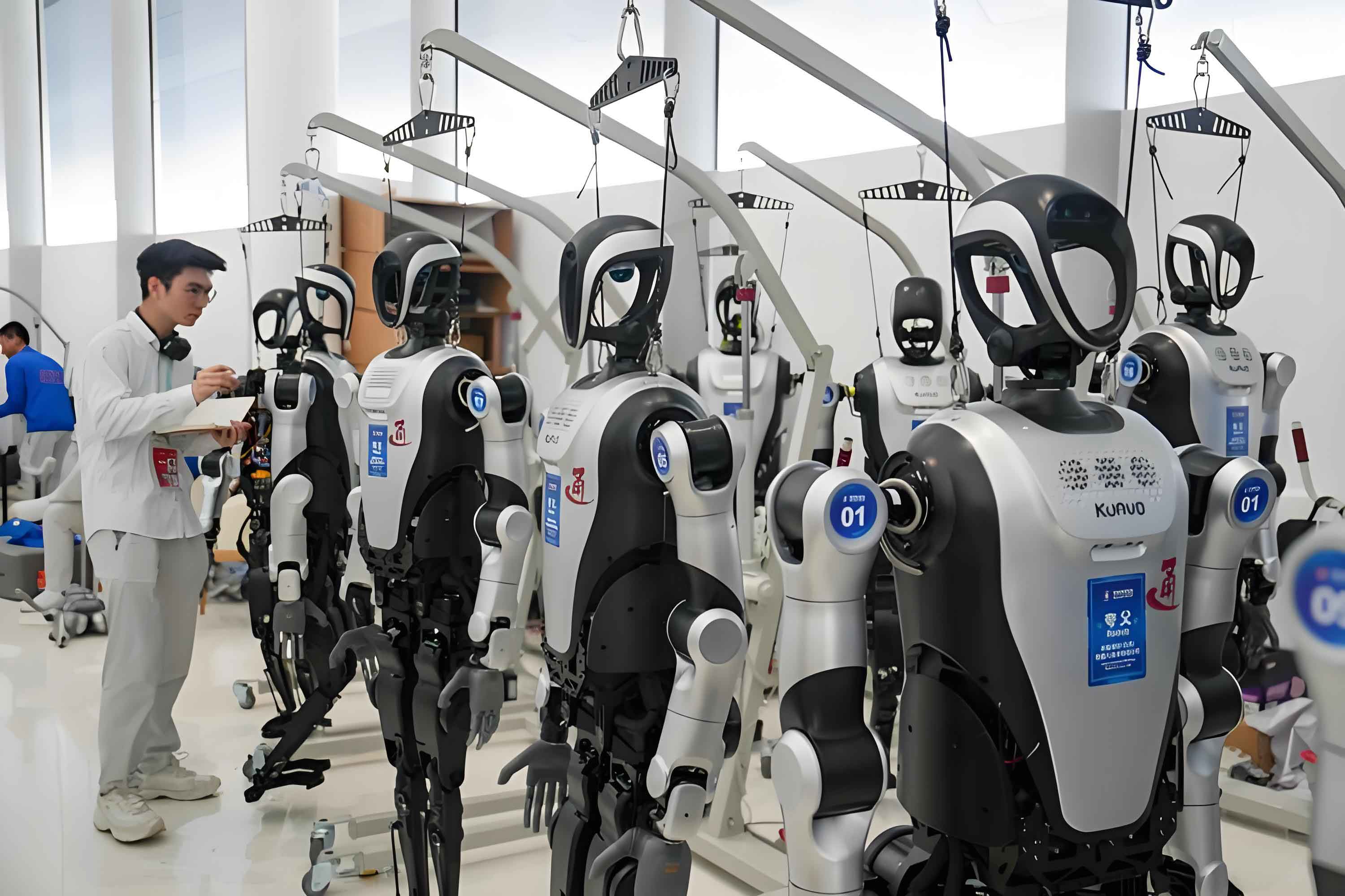
The position and orientation errors of the end effector are shown in Figure (refer to the attached photo of a humanoid robot in a quality inspection scenario). The errors converge to zero within approximately 24 seconds. The base moved from the origin to a final position around \( (1.0, 0.0, 0.0) \) m, while all joint positions remained within the prescribed limits.
6.3 Constraint Satisfaction
The base velocities and joint velocities are shown below. All velocities stayed below the assigned limits after an initial transient. The joint position trajectories were smooth and monotonic, indicating that the MPC produced feasible and executable commands.
To evaluate the tip-over prevention, I ran a comparative simulation with and without the CoG constraint. Without the constraint, the CoG eventually left the support polygon and the robot tipped over. With the constraint, the CoG remained inside the support circle throughout the entire task. The results are summarized in the following table.
| Constraint | CoG trajectory inside support circle | Task success |
|---|---|---|
| Without tip-over constraint | No | Fail (tip-over) |
| With tip-over constraint | Yes | Success |
6.4 Random Task Benchmark
I randomly sampled 50 target poses in front of the robot (x: 0.5–1.5 m, y: −0.75 to 0.75 m, z: 1.0–1.5 m; orientation uniformly sampled in SO(3)). The SLQ-MPC controller achieved a 96% success rate. The average task completion time was 14.2 seconds, and the average end-effector path length was 1.32 m. The two failures were due to unreachable target orientations near the boundary of the workspace; this can be mitigated by intermediate waypoint planning.
6.5 Physical Robot Validation
I deployed the SLQ-MPC controller on the physical robot. The controller ran on the Jetson Orin Nano at a frequency of 10 Hz, which was sufficient for real-time performance because the feedback gain computed by MPC was executed at 100 Hz between MPC updates. The robot successfully performed a whole-body manipulation task: it moved its base, torso, and arm simultaneously to place its end effector at a target position on a shelf while maintaining balance and avoiding self-collision. The experimental results matched the simulation, confirming the practical applicability of the proposed control method.
7. Conclusion and Future Work
In this thesis, I presented a complete whole-body motion control system for a wheeled humanoid robot. I designed the hardware and software architecture, derived the whole-body kinematics, and implemented two control strategies. The QP-based method with control barrier functions is effective for reactive manipulation but suffers from limited constraint handling and smoothness. The SLQ-MPC-based method provides a unified, real-time optimal control framework that explicitly handles joint position and velocity limits, collision avoidance, and tip-over prevention while achieving smooth trajectories and high task success rates. My experiments demonstrated that the MPC approach is both efficient and practical for real-world deployment of wheeled humanoid robots.
Future work will focus on extending the framework to bimanual manipulation, adding visual servoing to automatically obtain target poses from perception, and incorporating external obstacle avoidance using an Euclidean signed distance field. I also plan to explore learning-based models to accelerate the MPC computation and to adapt the controller to varying payloads and dynamic environments.