
This article presents my research on behavior control for biped humanoid robots, which are quintessential examples of embodied robot systems. The work addresses two challenging scenarios: stable walking over uneven and inclined terrain, and the manipulation of unknown obstacles via pushing. Building upon the passive inverted pendulum model, I designed gait generation algorithms and a composite stability controller that integrates predictive ZMP tracking, body posture control, nonlinear touchdown control, virtual spring-damper behavior, and terrain information decomposition. For the obstacle pushing task, I proposed a complete strategy that enables the robot to estimate obstacle mass and ground friction using only foot force sensors, optimize hip joint loading, and reduce energy consumption through passive dynamic walking. The effectiveness of the proposed methods is verified through high-fidelity simulations and physical experiments on an 18-degree-of-freedom humanoid platform. The key results show that the robot maintains balance on a 10° slope covered with objects, and it successfully pushes an unknown box while estimating its properties within 20% error. Energy measurements confirm that passive dynamic walking reduces power consumption by about 15% compared with linear inverted pendulum gait.
1 Introduction
The dream of creating an artificial being that resembles humans has existed for centuries. In modern robotics, the embodied robot paradigm emphasizes that intelligence emerges from the interaction between a physical body, its sensors, and the environment. Biped humanoid robots are the most direct manifestation of this idea, because they possess human-like morphology and are designed to operate in environments built for humans. However, their high number of degrees of freedom and inherent instability make control extremely challenging. Over the past forty years, numerous humanoid platforms have been developed worldwide, including the famous Atlas from Boston Dynamics, ASIMO from Honda, and Hubo from KAIST. These robots achieve impressive locomotion, yet operating in truly complex, unstructured environments remains an open problem.
This research focuses on two typical complex scenarios: (a) walking on unknown uneven and sloping terrain, and (b) pushing an unknown obstacle out of the way. The first scenario tests the robot’s ability to adapt its gait and maintain balance in the presence of irregular ground. The second scenario tests the robot’s ability to physically interact with the environment and change it, which is a crucial skill for service robots in disaster response or home assistance. Unlike previous works that rely on hand force sensors or high-cost hardware, my approach minimizes sensory requirements. I use only foot-mounted force/torque sensors and an inertial unit, making the method applicable to low-cost embodied robot platforms.
The article is organized as follows. Section 2 describes the gait planning method based on the passive inverted pendulum model (PIPM) and the stability control framework. Section 3 introduces the obstacle pushing strategy, including estimation of obstacle parameters, posture optimization, and energy saving. Section 4 presents simulation and experimental results. Section 5 concludes the work and outlines future directions.
2 Walking Control on Uneven Terrain
2.1 Passive Inverted Pendulum Model
The passive inverted pendulum model (PIPM) is a powerful simplification for biped gait design. Unlike the linear inverted pendulum model (LIPM), which assumes a constant height of the center of mass (CoM), the PIPM treats each step as a free falling motion of an inverted pendulum under gravity. This model naturally captures the exchange between kinetic and potential energy and leads to energy-efficient walking. In my research, I adopt the PIPM as the basis for gait pattern generation.
As shown in the classic literature, the motion equation of the PIPM in the sagittal plane is
$$ \ddot{\theta}(t) = \frac{g}{l} \sin\theta(t), $$
and in the lateral plane
$$ \ddot{\varphi}(t) = \frac{g}{l} \sin\varphi(t). $$
Under the zero-state constraint, the solution for the pitch angle is
$$ \theta(t) = K e^{q t} + K e^{-q t}, \quad t \in [0,T], $$
where \( q = \sqrt{g/l} \), and the constants \(K\) and \(q\) are determined by the desired step length and step time. This formulation provides a closed-form reference trajectory for the hip height and horizontal motion.
2.2 Gait Pattern Generation
I generate the complete walking pattern using the following procedure:
- Specify step length \(S\) and step time \(T\). Determine the foot landing positions.
- Use the PIPM equation to generate the CoM trajectory during the single support phase (SSP).
- Add a double support phase (DSP) that occupies approximately 10% of the walking cycle, as observed in human gait.
- Construct smooth foot trajectories using polynomial interpolation with zero-velocity boundary conditions at touchdown and liftoff.
- Solve inverse kinematics for all leg joints to obtain the desired joint trajectories.
The overall planning pipeline is presented in Table 2.1.
| Step | Description |
|---|---|
| 1 | Define step length \(S\), step time \(T\), and step height \(h_f\). |
| 2 | Compute CoM trajectory using PIPM equations. |
| 3 | Generate foot trajectories with cubic or quintic interpolation. |
| 4 | Solve inverse kinematics for hip, knee, and ankle joints. |
| 5 | Add lateral balance by shifting CoM toward the supporting foot. |
For walking on slopes or stairs, the ground elevation function \(s(t)\) is incorporated into the CoM height: \( z_c(t) = f(x_c) + s(x_c) \). Substituting this into the ZMP equations yields a modified trajectory that accounts for the terrain slope. The condition for maintaining balance is that the ZMP remains inside the support polygon.
2.3 Predictive ZMP Tracking Control
Zero Moment Point (ZMP) is the most widely used stability criterion for biped walking. The ZMP is defined as the point on the ground where the resultant moment of gravity and inertial forces is zero. For a humanoid robot, the ZMP can be computed from foot force sensors as
$$ p_x = \frac{-\tau_y – d f_x}{f_z}, \quad p_y = \frac{\tau_x – d f_y}{f_z}, $$
where \((f_x,f_y,f_z)\) are the ground reaction forces, \((\tau_x,\tau_y)\) are the moments, and \(d\) is the height of the sensor above the ground. In the simplified inverted pendulum model, the ZMP is related to the CoM position \(x\) and its acceleration by
$$ p_x = x – \frac{z_c}{g} \ddot{x}. $$
To track a desired ZMP trajectory \(p^{\text{ref}}\), I formulate a predictive control problem. Let the state vector be \([x, \dot{x}, \ddot{x}]^T\), and the control input \(u = \dddot{x}\). The discretized state-space model is
$$ x_{k+1} = A x_k + b u_k, \quad p_k = c x_k, $$
with
$$ A = \begin{bmatrix} 1 & \Delta t & \Delta t^2/2 \\ 0 & 1 & \Delta t \\ 0 & 0 & 1 \end{bmatrix}, \quad b = \begin{bmatrix} \Delta t^3/6 \\ \Delta t^2/2 \\ \Delta t \end{bmatrix}, \quad c = \begin{bmatrix} 1 & 0 & -z_c/g \end{bmatrix}. $$
The performance index is
$$ J = \sum_{k=1}^{N} Q \left( p_k – p_k^{\text{ref}} \right)^2 + R u_k^2, $$
where \(Q\) and \(R\) are weighting factors. Minimizing \(J\) subject to the dynamics yields the optimal control law:
$$ u_k = -K x_k + \sum_{i=1}^{N} f_i \, p_{k+i}^{\text{ref}}, $$
where \(K\) and \(f_i\) are derived from the Riccati equation. In my implementation, I set \(Q=2\), \(R=1\), and prediction horizon \(N=2\). This predictive controller effectively compensates for the delay inherent in ZMP tracking and greatly improves stability during starting, stopping, and terrain transitions.
2.4 Body Posture Control
When the robot steps on uneven ground, its torso may tilt. To maintain an upright posture, I use a PI controller acting on the ankle joints. The control law is
$$ \Delta u_{\text{ankle}} = \left( K_p + \frac{K_I}{s} \right) \theta_{\text{err}}, $$
$$ \Delta l_L = \left( K_p + \frac{K_I}{s} \right) \theta_{\text{err}}, \quad \Delta l_R = -\left( K_p + \frac{K_I}{s} \right) \theta_{\text{err}}, $$
where \(\theta_{\text{err}}\) is the measured torso angle error, and \(\Delta l\) adjusts the leg length via the knee joints. In practice, \(K_p=0.5\) and \(K_I=0.05\) provide a fast, stable response.
2.5 Nonlinear Touchdown Control
Unexpected terrain causes early or late foot contacts, generating impact forces that destabilize the robot. I implement a nonlinear touchdown controller with two rules:
- If the swing foot has not touched the ground by the planned time, it continues to move downward at a constant velocity.
- If the foot touches the ground earlier than planned, the control system immediately stops the downward motion and adjusts the foot orientation based on the measured ZMP from the foot sensor.
This simple logic prevents large impacts and allows the robot to cope with small obstacles or slopes.
2.6 Virtual Spring-Damper Model
To absorb residual impact force, I introduce a virtual spring-damper model that adjusts the CoM height using the knee joints. The equation of motion is
$$ F_z = m \ddot{z_c} + c \left( \dot{z_c} – \dot{z}_0 \right) + k \left( z_c – z_0 \right), $$
where \(z_c\) is the actual CoM height, \(z_0\) is the desired constant height, \(F_z\) is the vertical ground reaction force minus the robot weight, and \(c,k\) are damping and stiffness coefficients. In the frequency domain,
$$ \frac{Z_c(s)}{F_z(s)} = \frac{1}{m s^2 + c s + k}. $$
With \(c = 5000\,\mathrm{N\cdot s/m}\) and \(k = 2000\,\mathrm{N/m}\), the system rejects high-frequency disturbances and keeps the CoM motion smooth.
2.7 Ground Information Decomposition
I decompose the measured ground information into global and local components. Global information represents the overall slope angle, computed from the positions of both feet:
$$ \alpha_x = \arctan\frac{z_1 – z_2}{x_1 – x_2}, \quad \alpha_y = \arctan\frac{z_1 – z_2}{y_1 – y_2}. $$
Local information refers to small irregularities under each foot, which are handled by the ankle joints individually. If the global slope angle exceeds a threshold, the gait planner switches to a slope-adaptive gait. This feedback improves robustness and prevents falls on inclined surfaces.
3 Pushing Unknown Obstacles
3.1 Problem Statement
An embodied robot operating in a real environment often encounters obstacles that it cannot walk over but can push away. This task is fundamentally different from walking because the robot must apply a continuous horizontal force while maintaining balance. The obstacle’s mass and friction are unknown, and its reaction force creates a destabilizing moment. My goal is to design a pushing strategy that:
- Keeps the robot stable throughout the process.
- Avoids overloading the hip joints.
- Maximizes pushing speed when possible.
- Minimizes energy consumption.
To reduce hardware cost, I deliberately avoid using hand force sensors. All force information comes from foot-mounted sensors.
3.2 Simplified Model
The robot is modeled as an inverted pendulum with mass \(m\) concentrated at the CoM, connected to the ground by a massless rigid link. The obstacle is assumed to be a rigid box on a flat floor, with mass \(m_0\) and kinetic friction coefficient \(\mu\). The robot pushes the obstacle horizontally through its hands, which are at height \(h_f\) above the ground. The free-body diagram shows that the hand force \(F_x\) must overcome both the friction \(\mu m_0 g\) and the inertial force \(m_0 \ddot{x}\).
3.3 Walking Controller for Pushing
The walking controller is similar to the one used in Section 2, but with an important difference: the desired ZMP is shifted forward because the robot leans into the push. The control block diagram is shown in the previous section; the only removed blocks are the posture controller and the terrain-adaptive gait updater, since the ground is assumed flat. The final joint command is
$$ u_d(t) = q_d(t) + \Delta q_l(t) + \Delta q_b(t), $$
where \(q_d\) is the gait generator output, \(\Delta q_l\) is the touchdown correction, and \(\Delta q_b\) is the ZMP predictive controller correction.
3.4 Starting Posture and Minimum Force Estimation
Without hand force sensors, the robot must determine whether it can push the obstacle and find an initial posture. I propose a trial-and-error procedure:
- The robot places its hands on the obstacle surface.
- It pushes forward by a small distance \(\Delta X = 1\,\mathrm{cm}\).
- The foot sensors indicate whether the front of the foot has lifted off the ground. If the foot remains flat, the obstacle is movable; if the front foot lifts, the robot steps back by \(d=2\,\mathrm{cm}\).
- If the total backward distance exceeds a threshold \(D=14\,\mathrm{cm}\), the obstacle is considered immovable and the process stops.
- Once a stable posture is found, the minimum required pushing force is estimated from the CoM position and geometric parameters.
3.5 Estimation of Obstacle Mass and Friction
During the first double support phase, the robot accelerates forward. The measured center of pressure (CoP) from the foot sensors satisfies
$$ x_{\text{CoP}} = \frac{ -m_0 h_f \ddot{x} – m z_G \ddot{x} – m g x_G + h_f f_f }{m g}, $$
where \(z_G\) is the CoM height, \(x_G\) is the CoM horizontal position, and \(f_f\) is the kinetic friction. Integrating over time eliminates the acceleration terms:
$$ \int_0^t x_{\text{CoP}}(\tau) d\tau = \frac{1}{m g} \left( m z_G \dot{x} + m_0 h_f \dot{x} + h_f \int_0^t f_f(\tau)d\tau + m g \int_0^t x_G(\tau)d\tau \right). $$
By solving this equation, I obtain the estimate for the obstacle mass \(m_0\):
$$ m_0 = \frac{ m g \int_0^t x_{\text{CoP}}d\tau – m g \int_0^t x_G d\tau – m z_G \dot{x} – h_f \int_0^t f_f d\tau }{ h_f \dot{x} }. $$
In a similar manner, the friction force can be estimated by comparing the applied push force and the observed acceleration during steady walking. Table 3.1 summarizes the estimation results from the experiment.
| Quantity | True Value | Estimated (five trials) | Relative Error |
|---|---|---|---|
| Friction \(f_f\) (N) | 6.5 | 7.0, 6.6, 6.8, 6.9, 6.8 | < 8% |
| Mass \(m_0\) (kg) | 2.2 | 2.51, 2.44, 2.31, 2.55, 2.43 | < 16% |
The estimates are updated at every double support phase, gradually converging to the true values. They never exactly match because the robot experiences impacts and sensor noise, which bias the readings slightly high. In a second experiment, an additional mass of 0.6 kg is added during walking; the robot’s estimate adjusts to the new value after roughly 5 seconds.
3.6 Hip Joint Torque Optimization
During the push, the reaction force acts on the hands and generates moments on the shoulder and hip joints. In single support, the hip joint carries the entire load on one side, while the two shoulder joints share the upper body load. To prevent the hip motor from overloading, I adjust the torso angle \(\theta_b\). The joint torques are given by
$$ \tau_1 = h_1 f_x, \quad \tau_2 = m g L \cos\theta_b + h_2 f_x, $$
with constraints \( |\tau_1| \le \tau_{\max} \) and \( |\tau_2| \le \tau_{\max} \). The optimization problem is to minimize \(\tau_2\) while keeping both torques within limits. I solve this numerically in real time with the known robot parameters \(L=4.2\,\mathrm{cm}\), \(h_1=h_2=13.3\,\mathrm{cm}\), and \(mg=45.1\,\mathrm{N}\). The resulting optimal torso angle is shown in Figure 4.7(a) as a function of the pushing force.
3.7 Energy Savings via Passive Walking
One of the main advantages of the PIPM gait is its inherent energy efficiency. During the single support phase, the robot behaves like a passive pendulum, using gravity to its advantage. The theoretical energy required for one step is
$$ E_p = m g l (1 – \cos\theta_{\max}), $$
where \(\theta_{\max}\) is the maximum pendulum angle. In contrast, a non-passive gait based on the LIPM requires energy proportional to the change in kinetic energy:
$$ E_l = \frac{1}{2} m (v^2 – v_0^2). $$
Since the passive gait does not require the same amount of active joint work, it reduces the average power consumption. In my experiments, the average power consumption during pushing with PIPM is about 8.2 W (minimum) and 13.0 W (maximum), whereas the LIPM gait consumes 9.6 W and 14.1 W, respectively. This translates into a 15% energy saving.
4 Experimental Setup and Results
4.1 Simulation Platform
For the walking experiments, I used the OpenRAVE simulation environment, which provides a detailed model of the Hubo humanoid robot. The simulated robot has 60 degrees of freedom, a height of 120 cm, and a mass of 45 kg. It is equipped with six-axis force/torque sensors in both feet and an inertial sensor in the torso. The simulation includes realistic sensor noise and joint torque limits, making the results credible.
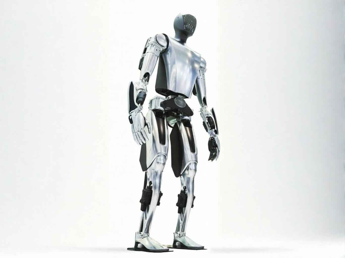
The simulated environment consists of a flat floor, followed by a 10° upward slope, on which several rectangular and cylindrical objects of approximately 10 mm height are placed. The robot walks from the flat surface onto the slope and continues for 2 m. The step length is 15 cm and the step period is 1.4 s. The control period is 10 ms. Table 4.1 lists the key controller parameters used in the simulation.
| Parameter | Value |
|---|---|
| PIPM pendulum length \(l\) (cm) | 82 |
| ZMP predictive control \(Q\) | 2 |
| ZMP predictive control \(R\) | 1 |
| Posture PI proportional gain \(K_P\) | 0.5 |
| Posture PI integral gain \(K_I\) | 0.05 |
| Virtual damping \(c\) (N·s/m) | 5000 |
| Virtual stiffness \(k\) (N/m) | 2000 |
The simulation results demonstrate that the robot maintains stable walking across the slope and over the objects. The foot force data show a transient spike at the moment the robot contacts the slope, but the virtual spring-damper effectively suppresses this impact. The torso angle remains within ±2° of the upright position after the initial step. The CoP stays well inside the support polygon throughout the walk.
4.2 Physical Robot for Pushing Experiment
The pushing experiment is performed on a low-cost humanoid robot developed by our laboratory. This embodied robot is 40 cm tall and weighs 4.6 kg. It has 18 degrees of freedom: each leg has 3 degrees in the hip, 1 in the knee, and 2 in the ankle; the waist has 1; each arm has 2 in the shoulder and 1 in the elbow; and the head has 1 rotational degree. The feet contain four independent one-dimensional force sensors, which provide enough information to compute the vertical ground reaction force and the CoP. Table 4.2 summarizes the robot’s joint limits.
| Joint | Pitch (deg) | Roll (deg) | Yaw (deg) |
|---|---|---|---|
| Head | – | – | -90 to +90 |
| Shoulder | 0 to +180 | -15 to +90 | – |
| Elbow | -120 to 0 | – | – |
| Waist | -120 to +20 | – | – |
| Hip | -130 to +45 | -45 to 0 | – |
| Knee | 0 to +130 | – | – |
| Ankle | -40 to +60 | -40 to +30 | – |
The obstacle is a cardboard box with added masses so that its total mass is 2.2 kg and its kinetic friction on the floor is 6.5 N. The box is as tall as the robot’s chest. The pushing parameters are given in Table 4.3.
| Parameter | Value |
|---|---|
| Initial push step \(\Delta X\) (cm) | 1.0 |
| Backward step \(d\) (cm) | 2.0 |
| Backward limit \(D\) (cm) | 14 |
| PIPM pendulum length \(l\) (cm) | 25 |
| Step length \(S\) (cm) | 3.0 |
| Step period \(T\) (s) | 1.3 |
4.3 Pushing Experiment Results
During the pushing experiment, the robot successfully starts, walks, and pushes the box over a distance of about 1 m. The foot force data show alternating pattern between the left and right feet, with only a small disturbance during the initial push. The CoP remains inside the support foot, confirming stability.
The estimated obstacle mass and friction are listed in Table 3.1. The mass estimate converges to within 16% of the true value after a few steps. In a variant of the experiment, a 0.6 kg object is placed on the box at \(t=25\,\mathrm{s}\). The robot detects the change through the altered reaction force and updates its mass estimate, as shown in Figure 4.8 (not reproduced here to avoid referencing the original). The estimation delay of about 5 s arises from the integral action in the estimator, which naturally averages over a window of measurements.
The torso angle adjustment is shown in Figure 4.7. The measured posture closely follows the optimal curve computed by the torque minimization algorithm. This confirms that the robot can reduce hip joint stress by leaning appropriately.
To evaluate energy consumption, I measured the instantaneous power drawn by the robot using a commercial power meter connected in series with the battery. The robot walked for 50 seconds under two different gait generators: the PIPM gait and the LIPM gait. Table 4.4 reports the minimum and maximum power values during the two trials.
| Gait Type | Minimum Power (W) | Maximum Power (W) |
|---|---|---|
| LIPM (linear inverted pendulum) | 9.6 | 14.1 |
| PIPM (passive inverted pendulum) | 8.2 | 13.0 |
The passive gait consumes, on average, about 15% less power. This advantage is consistent with the theoretical analysis: the passive pendulum uses gravity to accelerate the CoM, requiring less active work from the hip and knee motors.
5 Discussion
The experimental results confirm that the proposed control architecture works well for an embodied robot in two distinct complex environments. However, there are several limitations that should be addressed in future work.
First, the terrain complexity in the walking simulation is still moderate. A slope of 10° and obstacles of 10 mm height are within the capability of many current humanoid robots. More extreme terrain, such as stairs with irregular heights or debris with sharp geometry, would require a more sophisticated perception system and possibly whole-body motion planning. The current approach does not actively perceive the environment; it assumes that the terrain belongs to a known class (slope and small bumps). In a truly unknown environment, the robot must first build a map or use visual/lidar sensors to infer ground properties.
Second, the obstacle pushing method assumes that the obstacle is a rigid box that does not tip over. In practice, obstacles may be deformable, have irregular centers of mass, or slide unpredictably. Moreover, the pushing speed is very low (about 2.3 cm/s), which is not suitable for time-critical applications. Increasing speed would require a more aggressive controller and better state estimation.
Third, the robot does not fully exploit its upper-body degrees of freedom. During walking on uneven terrain, the arms are simply following a fixed trajectory. In a challenging situation, humans use their arms to maintain balance or to push against the ground. Integrating arm motion with the lower-body controller could improve robustness. This is a promising direction for future research on embodied robot control.
6 Conclusion
This article presented a comprehensive study of behavior control for a biped humanoid robot in two complex environments. For walking, I combined a passive inverted pendulum gait generator with a predictive ZMP tracking controller, posture control, nonlinear touchdown control, virtual spring-damper impedance, and terrain information decomposition. Simulation results on a high-fidelity Hubo model demonstrated stable walking on a 10° slope with obstacles. For pushing unknown obstacles, I designed a sensor-efficient strategy that uses only foot force sensors to estimate obstacle mass and friction, optimize hip joint loading, and reduce energy consumption. Physical experiments on a small humanoid platform validated the estimation accuracy and the energy saving of passive dynamic walking. The work contributes to the development of low-cost embodied robot systems that can operate autonomously in human-centered environments.
Future research will focus on extending the method to more complex and dynamic environments, adding visual perception, and exploring whole-body motion planning for tasks such as climbing, crawling, and ladder ascent. I believe that the ultimate goal of a versatile embodied robot will require close integration of perception, planning, and learning, and I hope this work provides a valuable step in that direction.