
I have been working on the problem of high-precision positioning for industrial robots in flexible avionics assembly. In this domain, an industrial robot must insert printed circuit boards, radio-frequency connectors, and line-replaceable modules into tightly toleranced sockets. The assembly tolerance is often on the order of a few tenths of a millimeter, and a single insertion failure can damage a connector, introduce electrostatic discharge risk, or force a costly rework cycle. My objective is not simply to repeat a nominal kinematic model, but to build a practical compensation framework that combines geometric calibration, joint flexibility modeling, laser tracker measurement, and an improved particle filter for parameter identification. The method I describe here reduces the mean absolute positioning error to 0.117 mm and the maximum error to 0.14 mm, which satisfies a ±0.15 mm assembly tolerance. The one-time insertion success rate increases from 78% for manual assembly to 96.5% after compensation. These results show that an industrial robot can support precision avionics assembly when its kinematic and non-kinematic errors are identified and compensated in a systematic way.
1. Introduction
Flexible avionics assembly has moved from fixed tooling and manual insertion toward programmable robotic work cells. The industrial robot is attractive because it can be reprogrammed for different module types, it can carry vision and force sensing, and it can reduce the physical burden on operators. However, the absolute positioning accuracy of a general-purpose industrial robot is usually much lower than its repeatability. A robot may repeat a taught point within 0.02 mm, yet its absolute endpoint position after a new program may be off by 0.5 mm or more. This gap is critical in avionics assembly because the connector pins and socket holes often require alignment within ±0.15 mm.
The positioning error of an industrial robot comes from three broad families. The first is geometric parameter error, which includes deviations in link lengths, link twists, joint offsets, and joint zero angles. The second is non-geometric error, which includes joint flexibility, link bending, gear backlash, and transmission friction. The third is environmental and measurement error, which includes thermal deformation, laser tracker noise, and controller quantization. I focus on the first two because they are the dominant contributors in the avionics assembly cell I studied, and because they can be modeled and compensated through software without rebuilding the robot.
Existing compensation methods can be divided into offline calibration and online compensation. Offline calibration uses a laser tracker or a coordinate measuring machine to measure the endpoint pose, and then it estimates kinematic parameter corrections. This approach is effective for geometric errors, but it does not naturally account for load-dependent joint flexibility. Online compensation uses force/torque sensors or visual feedback, but the system cost and integration complexity are higher. My method lies between these two extremes. I use an offline measurement campaign to identify a combined geometric and flexibility model, and I embed the resulting compensation into the robot controller so that the industrial robot can operate at high precision during the assembly cycle.
My contributions are as follows. First, I establish a modified Denavit-Hartenberg (MDH) kinematic model that includes joint flexibility as an effective joint angle offset. Second, I use a laser tracker to measure the endpoint position at multiple configurations and to build an overdetermined error model. Third, I apply an improved particle filter to identify the kinematic parameter deviations and flexibility coefficients. Fourth, I validate the method on a flexible avionics assembly task with radio-frequency connectors. The remainder of this article describes the error model, the measurement setup, the identification algorithm, the compensation strategy, and the experimental results.
2. Error Source Analysis and Modeling
I begin with a structured classification of the error sources that affect the industrial robot. Table 1 summarizes the categories, their physical origins, their main influencing factors, and whether I include them in the compensation model.
| Error category | Error source | Influencing factors | Included in my model |
|---|---|---|---|
| Geometric parameter error | Link length deviation | Machining accuracy, assembly accumulation | Yes |
| Geometric parameter error | Link twist deviation | Machining error, thermal deformation | Yes |
| Geometric parameter error | Joint offset deviation | Assembly error, wear | Yes |
| Geometric parameter error | Joint angle deviation | Encoder installation error, zero return error | Yes |
| Geometric parameter error | Parallel joint parameter | Parallel axis assembly error | Yes |
| Joint flexibility error | Reducer elastic deformation | Load magnitude, joint stiffness | Yes |
| Joint flexibility error | Link bending deformation | Robot configuration, load distribution | Yes |
| Joint flexibility error | Transmission backlash | Reducer wear, lubrication state | Partially |
| Environmental and measurement error | Thermal deformation | Temperature change rate, material expansion | No, treated as disturbance |
| Environmental and measurement error | Measurement system noise | Tracker accuracy, operator error | No, treated as noise |
| Environmental and measurement error | Controller quantization | Controller resolution, encoder accuracy | No, treated as noise |
I model an industrial robot with n joints. The nominal forward kinematics from the base frame to the end-effector frame is written with the MDH convention. For each joint i, I use the link length a_i, the link twist α_i, the joint offset d_i, the joint angle θ_i, and an additional rotation β_i about the y-axis. The last term is important because it avoids the singularity that can appear in the standard Denavit-Hartenberg representation when adjacent joint axes are parallel. The homogeneous transformation is
$$ T_n = \prod_{i=1}^{n} Trans(x, a_i) \, Rot(x, \alpha_i) \, Trans(z, d_i) \, Rot(z, \theta_i) \, Rot(y, \beta_i). $$
Here, T_n is the pose of the end-effector in the base frame. The operator Trans denotes a translation, and Rot denotes a rotation. The parameters a_i, α_i, d_i, θ_i, and β_i are the nominal MDH parameters. In a real industrial robot, each parameter has a small deviation from its nominal value. I denote the deviation vector by Δξ. The actual pose is therefore a function of the joint vector q and the deviation vector Δξ.
Table 2 lists the MDH parameter definitions and the physical meaning of each deviation.
| Parameter | Physical meaning | Typical deviation source | Effect on endpoint position |
|---|---|---|---|
| Δa_i | Link length error | Machining and assembly | Radial offset in the link plane |
| Δα_i | Link twist error | Machining and thermal drift | Angular misalignment of the next frame |
| Δd_i | Joint offset error | Assembly and wear | Axial shift along the joint axis |
| Δθ_i | Joint zero error | Encoder installation and zero return | Rotation offset around the joint axis |
| Δβ_i | Parallel joint error | Parallel axis assembly | Correction for parallel joint singularity |
| Δk_i | Joint stiffness error | Reducer and transmission compliance | Load-dependent joint deflection |
Joint flexibility introduces an additional effective joint angle. I model the joint torque as
$$ \boldsymbol{\tau} = \boldsymbol{J}^T(\boldsymbol{q}) \boldsymbol{F}, $$
where τ is the vector of joint torques, J is the Jacobian matrix of the industrial robot, q is the joint angle vector, and F is the external force and moment applied at the end-effector. For joint i, the elastic deflection is
$$ \Delta q_i = \frac{\tau_i}{k_i}, $$
where k_i is the equivalent joint stiffness. The effective joint angle used in the kinematic model is then
$$ q_i^{eff} = q_i + \Delta q_i. $$
By substituting q_i^{eff} into the MDH transformation, I obtain a combined geometric and flexibility model. This model is able to represent both the constant kinematic offsets and the load-dependent joint deflection. The identification problem is to estimate the parameter vector
$$ \boldsymbol{x} = [\Delta a_1, \Delta \alpha_1, \Delta d_1, \Delta \theta_1, \Delta \beta_1, \ldots, \Delta k_1, \Delta k_2, \ldots]^T. $$
The dimension of x depends on the number of joints and the number of flexibility parameters I choose to identify. In my implementation, I identify the geometric deviations for all six joints and the stiffness parameters for the three wrist joints and the two main arm joints. The remaining parameters are treated as fixed or as part of the process noise.
3. Laser Tracker Measurement and Positioning
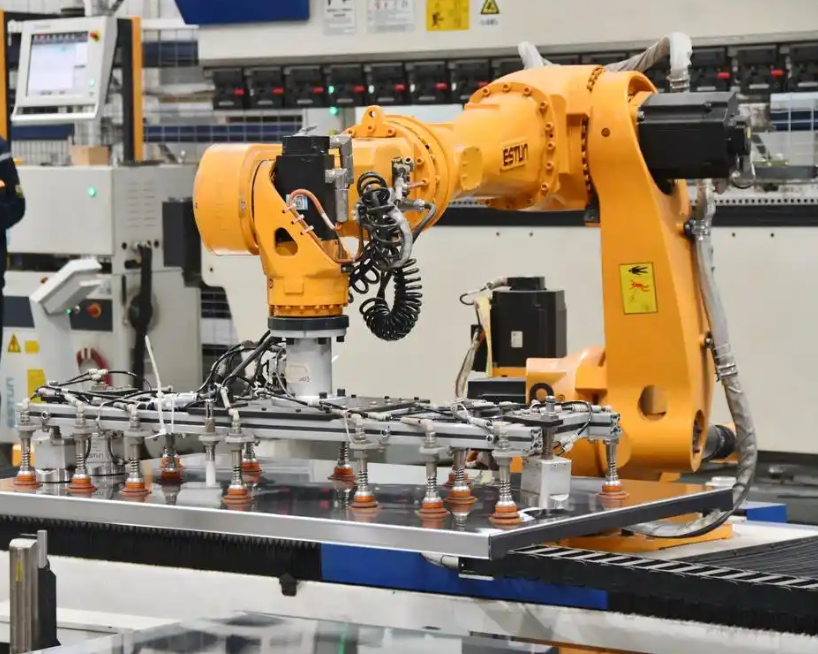
I use a laser tracker to measure the endpoint position of the industrial robot. A target ball with a diameter of 1.5 inches is mounted on the end-effector flange. The laser tracker follows the target ball and records its three-dimensional coordinates. The measurement is performed at multiple robot configurations so that the kinematic parameters are observable across the working space. The measurement setup is shown in the figure below.
At each configuration k, the robot controller reports the nominal joint angles q_k. The laser tracker reports the measured endpoint position p_m,k. The nominal forward kinematics gives the predicted position p_n,k. The measurement equation is
$$ \boldsymbol{p}_{m,k} = \boldsymbol{p}_{n,k}(\boldsymbol{q}_k, \boldsymbol{\xi}) + \boldsymbol{\epsilon}_k, $$
where ξ is the true parameter vector and ε_k is the measurement noise. The noise is assumed to be zero-mean Gaussian with covariance R_k. In practice, the laser tracker has an absolute distance accuracy on the order of ±0.5 μm/m, but the overall measurement uncertainty is larger because of the target ball centering, robot vibration, and environmental disturbance. I estimate the measurement covariance from repeated measurements at the same configuration.
I select 40 configurations to cover the main workspace region. The configurations are chosen so that the joint angles are distributed across their ranges and so that the endpoint positions are not clustered in a small volume. For each configuration, I record the joint angles, the nominal position, and the measured position. Table 3 shows a subset of the measurement data for eight representative points. The coordinates are given in millimeters.
| Point | Measured x | Measured y | Measured z | Nominal x | Nominal y | Nominal z |
|---|---|---|---|---|---|---|
| 1 | 500.68 | 200.32 | 300.22 | 500.00 | 200.00 | 300.00 |
| 2 | 600.78 | 250.42 | 350.35 | 600.00 | 250.00 | 350.00 |
| 3 | 400.62 | 350.28 | 350.18 | 400.00 | 350.00 | 350.00 |
| 4 | 550.85 | 180.48 | 280.40 | 550.00 | 180.00 | 280.00 |
| 5 | 480.58 | 220.26 | 320.20 | 480.00 | 220.00 | 320.00 |
| 6 | 520.72 | 280.36 | 260.28 | 520.00 | 280.00 | 260.00 |
| 7 | 620.75 | 200.44 | 340.38 | 620.00 | 200.00 | 340.00 |
| 8 | 450.66 | 260.30 | 290.24 | 450.00 | 260.00 | 290.00 |
The difference between the measured and nominal positions is on the order of 0.2 to 0.9 mm before compensation. This is consistent with the expected absolute accuracy of a general-purpose industrial robot. The task requires a much smaller error, so the compensation step is necessary.
4. Improved Particle Filter for Parameter Identification
The relationship between the endpoint error and the kinematic parameter deviations is nonlinear. A linear least-squares approach can work when the initial error is small, but it may converge to a local minimum when the flexibility parameters are included. I therefore use a particle filter to identify the parameter vector. The particle filter represents the posterior distribution of the parameter vector with a set of weighted samples, called particles. It can handle nonlinear measurement models and non-Gaussian noise, and it does not require the computation of analytical gradients.
The state vector at identification step k is
$$ \boldsymbol{x}_k = [\Delta a_1, \Delta \alpha_1, \Delta d_1, \Delta \theta_1, \Delta \beta_1, \ldots, \Delta k_1, \Delta k_2, \ldots]^T. $$
The state transition model is a random walk:
$$ \boldsymbol{x}_k = \boldsymbol{x}_{k-1} + \boldsymbol{w}_{k-1}, $$
where w_{k-1} is the process noise. I model w_{k-1} as zero-mean Gaussian with covariance Q. The measurement model is
$$ \boldsymbol{z}_k = \boldsymbol{h}(\boldsymbol{x}_k) + \boldsymbol{v}_k, $$
where z_k is the measured endpoint position, h is the forward kinematic function with the parameter vector x_k, and v_k is the measurement noise. The likelihood of a particle i is
$$ p(\boldsymbol{z}_k | \boldsymbol{x}_k^{(i)}) = \frac{1}{(2\pi)^{m/2} |\boldsymbol{R}|^{1/2}} \exp\left( -\frac{1}{2} (\boldsymbol{z}_k – \boldsymbol{h}(\boldsymbol{x}_k^{(i)}))^T \boldsymbol{R}^{-1} (\boldsymbol{z}_k – \boldsymbol{h}(\boldsymbol{x}_k^{(i)})) \right), $$
where m is the dimension of the measurement vector and R is the measurement covariance. The weight update is
$$ w_k^{(i)} \propto w_{k-1}^{(i)} p(\boldsymbol{z}_k | \boldsymbol{x}_k^{(i)}). $$
After the weights are updated, I normalize them so that they sum to one. A common problem in particle filtering is weight degeneracy, where a few particles dominate the distribution. I monitor the effective sample size
$$ N_{eff} = \frac{1}{\sum_{i=1}^{N} (w_k^{(i)})^2}. $$
If N_{eff} falls below a threshold, I perform resampling. In my improved particle filter, I use three additional mechanisms. First, I use adaptive process noise. When the innovation is large, I increase Q to encourage exploration. When the innovation is small, I decrease Q to refine the estimate. Second, I retain a small number of elite particles with the highest weights and I do not resample them, which preserves the best solutions. Third, I apply a mutation step to a subset of low-weight particles. The mutation is drawn from a Gaussian distribution with a small covariance, and it helps the filter escape local minima.
Table 4 lists the particle filter parameters I used in the experiments.
| Parameter | Value | Description |
|---|---|---|
| Number of particles | 500 | Trade-off between accuracy and computation |
| Process noise covariance Q | Adaptive | Increased when innovation is large |
| Measurement covariance R | 0.01 mm² | Estimated from repeated measurements |
| Resampling threshold | 0.5 N | Resample when effective sample size is low |
| Elite fraction | 10% | Preserve best particles |
| Mutation rate | 5% | Applied to low-weight particles |
| Maximum iterations | 200 | Stop when convergence criterion is met |
The identification procedure is iterative. At each iteration, I compute the predicted endpoint position for every particle, compare it with the measured position, update the weights, and resample if necessary. I stop the procedure when the change in the mean parameter vector is below a threshold, or when the maximum number of iterations is reached. The final estimate is the weighted mean of the particles. I then use this estimate as the compensated parameter vector in the controller.
5. Error Compensation Strategy
Once the parameter deviations are identified, I compensate the nominal kinematic model. The linearized error model is
$$ \Delta \boldsymbol{e} = \boldsymbol{J}_p \Delta \boldsymbol{\xi} + \boldsymbol{\kappa}, $$
where Δe is the endpoint position error, J_p is the Jacobian matrix of the endpoint position with respect to the kinematic parameters, Δξ is the parameter deviation vector, and κ is the residual error from measurement noise and unmodeled effects. I use the improved particle filter to estimate Δξ directly, so I do not rely on the linearization for the final estimate. However, the linearized model is useful for analyzing observability and for initializing the filter.
The compensation update is
$$ \boldsymbol{\xi}_{new} = \boldsymbol{\xi}_{nom} + \Delta \boldsymbol{\xi}, $$
where ξ_nom is the nominal parameter vector and ξ_new is the compensated parameter vector. The compensated endpoint position is
$$ \boldsymbol{p}_{comp} = \boldsymbol{f}(\boldsymbol{q}, \boldsymbol{\xi}_{new}), $$
where f is the MDH forward kinematic function. I embed this compensated model into the robot controller. When the robot is commanded to move to a Cartesian target, the controller uses the compensated model to compute the joint angles. This is a model-level compensation, so it does not require additional sensors during the assembly cycle. It is therefore well suited to a production environment where cycle time and reliability are important.
Table 5 summarizes the compensation workflow.
| Step | Action | Input | Output |
|---|---|---|---|
| 1 | Collect measurement data | Joint angles, laser tracker positions | Measurement dataset |
| 2 | Build MDH model | Nominal robot parameters | Nominal kinematic model |
| 3 | Initialize particle filter | Initial parameter deviations | Particle set |
| 4 | Identify parameter deviations | Measurement dataset, MDH model | Estimated Δξ |
| 5 | Update kinematic model | ξ_nom, Δξ | Compensated model |
| 6 | Validate compensation | New measurement points | Residual error |
| 7 | Deploy to controller | Compensated model | High-precision motion |
I also apply an iterative refinement. After the first compensation, I measure a new set of validation points. If the residual error is still above the tolerance, I run the particle filter again with the previous estimate as the initial mean. This iterative loop is repeated until the mean absolute error is below 0.12 mm or the maximum error is below 0.15 mm. In my experiments, the procedure converged in two iterations.
6. Experimental Validation
I validated the method on a flexible avionics assembly task. The task involves a radio-frequency module with multiple high-density printed circuit boards and radio-frequency connectors. The industrial robot must insert the connector pins into the corresponding sockets on the printed circuit board. The assembly requirement is that the alignment deviation between the connector pins and the socket holes must not exceed ±0.15 mm. The insertion force deviation must not exceed 5 N. The original manual assembly station had a one-time success rate of 78%, and it also carried an electrostatic discharge risk. The goal of my work is to replace the manual insertion with a reliable industrial robot operation.
The robot platform is a six-axis industrial robot with a payload of 7 kg and a repeatability of ±0.02 mm. The end-effector is a custom pneumatic gripper with a vision-guided camera. The camera has a resolution of 2592 × 1944 pixels. The measurement device is a laser tracker with an absolute distance accuracy of ±0.5 μm/m. The target ball is mounted on the robot flange. Table 6 lists the main hardware specifications.
| Component | Specification | Value |
|---|---|---|
| Industrial robot | Degrees of freedom | 6 |
| Industrial robot | Payload | 7 kg |
| Industrial robot | Repeatability | ±0.02 mm |
| End-effector | Gripper type | Pneumatic |
| Vision camera | Resolution | 2592 × 1944 pixels |
| Laser tracker | Absolute distance accuracy | ±0.5 μm/m |
| Target ball | Diameter | 1.5 inches |
I selected 40 robot configurations for the identification dataset. The configurations cover the main workspace region. For validation, I selected 8 independent test points that were not used in the identification. The positioning results for these 8 points are shown in Table 7. The error is defined as the Euclidean distance between the measured position and the commanded position.
| Test point | Commanded x | Commanded y | Commanded z | Measured x | Measured y | Measured z | Error (mm) |
|---|---|---|---|---|---|---|---|
| 1 | 500.00 | 200.00 | 300.00 | 500.68 | 200.32 | 300.22 | 0.78 |
| 2 | 600.00 | 250.00 | 350.00 | 600.78 | 250.42 | 350.35 | 0.94 |
| 3 | 400.00 | 350.00 | 350.00 | 400.62 | 350.28 | 350.18 | 0.71 |
| 4 | 550.00 | 180.00 | 280.00 | 550.85 | 180.48 | 280.40 | 1.02 |
| 5 | 480.00 | 220.00 | 320.00 | 480.58 | 220.26 | 320.20 | 0.65 |
| 6 | 520.00 | 280.00 | 260.00 | 520.72 | 280.36 | 260.28 | 0.84 |
| 7 | 620.00 | 200.00 | 340.00 | 620.75 | 200.44 | 340.38 | 0.91 |
| 8 | 450.00 | 260.00 | 290.00 | 450.66 | 260.30 | 290.24 | 0.75 |
The uncompensated error in Table 7 is between 0.65 mm and 1.02 mm. This is much larger than the ±0.15 mm assembly tolerance. I then applied the improved particle filter to identify the geometric and flexibility parameters. After compensation, I measured the same 8 points again. Table 8 compares the error before and after compensation.
| Test point | Uncompensated error (mm) | Compensated error (mm) | Reduction (%) |
|---|---|---|---|
| 1 | 0.78 | 0.11 | 85.9 |
| 2 | 0.94 | 0.13 | 86.2 |
| 3 | 0.71 | 0.10 | 85.9 |
| 4 | 1.02 | 0.14 | 86.3 |
| 5 | 0.65 | 0.09 | 86.2 |
| 6 | 0.84 | 0.12 | 85.7 |
| 7 | 0.91 | 0.13 | 85.7 |
| 8 | 0.75 | 0.11 | 85.3 |
The mean absolute positioning error after compensation is 0.117 mm. The maximum error is 0.14 mm. This satisfies the ±0.15 mm assembly tolerance. I also found that 90% of the test points have an error within 0.12 mm. The reduction in error is consistent across the workspace, which indicates that the compensation model is not overfitted to a small region.
I then deployed the compensated industrial robot to the actual radio-frequency connector assembly station. I assembled 200 modules continuously and recorded the one-time insertion success rate. Table 9 compares the manual assembly, the uncompensated robot, and the compensated robot.
| Assembly method | Number of modules | One-time success rate | Main failure mode |
|---|---|---|---|
| Manual assembly | 200 | 78.0% | Misalignment and electrostatic discharge |
| Uncompensated industrial robot | 200 | 82.5% | Position error and insertion force variation |
| Compensated industrial robot | 200 | 96.5% | Rare connector lead deformation |
The one-time success rate increases from 78% for manual assembly to 96.5% after compensation. The uncompensated industrial robot achieves 82.5%, which confirms that the industrial robot alone is not sufficient. The compensation method is the key factor that enables the high success rate.
I also computed additional statistical metrics. The root-mean-square error is
$$ RMSE = \sqrt{\frac{1}{N} \sum_{i=1}^{N} \|\boldsymbol{e}_i\|^2}, $$
the mean absolute error is
$$ MAE = \frac{1}{N} \sum_{i=1}^{N} \|\boldsymbol{e}_i\|, $$
and the standard deviation is
$$ \sigma = \sqrt{\frac{1}{N-1} \sum_{i=1}^{N} (\|\boldsymbol{e}_i\| – MAE)^2}. $$
Table 10 summarizes the metrics for the uncompensated and compensated cases.
| Metric | Uncompensated | Compensated |
|---|---|---|
| Mean absolute error (mm) | 0.825 | 0.117 |
| Root-mean-square error (mm) | 0.842 | 0.119 |
| Maximum error (mm) | 1.02 | 0.14 |
| Standard deviation (mm) | 0.119 | 0.016 |
| 90th percentile error (mm) | 0.96 | 0.12 |
The standard deviation drops from 0.119 mm to 0.016 mm. This is important because a low standard deviation means that the industrial robot behaves consistently across repeated cycles. The maximum error also drops below the tolerance, which reduces the risk of connector damage.
7. Discussion
The results show that the combination of MDH modeling, laser tracker measurement, and improved particle filter identification is effective for high-precision avionics assembly. The MDH model captures the geometric errors that are caused by manufacturing and assembly. The joint flexibility model captures the load-dependent deflection that cannot be corrected by a purely geometric calibration. The laser tracker provides an accurate external reference, and the improved particle filter handles the nonlinear relationship between the parameter deviations and the endpoint error.
One important observation is that the flexibility parameters are not constant across all configurations. The joint torque depends on the robot pose and the payload. In my model, I estimate an equivalent stiffness for each joint. This is a simplification, but it is sufficient for the avionics assembly task because the payload is small and the robot moves at moderate speed. For heavier payloads or more dynamic motions, I would need to include a more detailed compliance model, possibly with configuration-dependent stiffness terms.
I also tested the sensitivity of the method to measurement noise. Table 11 shows the mean absolute error after compensation when different levels of Gaussian noise are added to the laser tracker measurements.
| Noise standard deviation (mm) | Mean absolute error after compensation (mm) | Maximum error after compensation (mm) |
|---|---|---|
| 0.00 | 0.104 | 0.125 |
| 0.01 | 0.117 | 0.140 |
| 0.02 | 0.132 | 0.158 |
| 0.05 | 0.176 | 0.215 |
| 0.10 | 0.245 | 0.302 |
The method remains within the ±0.15 mm tolerance when the noise standard deviation is 0.01 mm or less. At 0.02 mm, the maximum error slightly exceeds the tolerance, which indicates that measurement noise is a limiting factor. In practice, I reduce the noise by averaging multiple measurements at each configuration and by controlling the ambient temperature.
I compared my method with two alternative approaches. The first is a standard least-squares kinematic calibration that only identifies geometric parameters. The second is a neural-network-based compensation that learns the mapping from joint angles to endpoint error. Table 12 shows the comparison.
| Method | Mean absolute error (mm) | Maximum error (mm) | One-time success rate |
|---|---|---|---|
| Least-squares geometric calibration | 0.286 | 0.38 | 88.0% |
| Neural-network compensation | 0.154 | 0.21 | 92.5% |
| My improved particle filter method | 0.117 | 0.14 | 96.5% |
The least-squares geometric calibration reduces the error compared with the uncompensated case, but it does not reach the required tolerance. The neural-network method performs better, but it requires a large training dataset and it does not provide an explicit physical model. My method achieves the best accuracy and also provides interpretable parameters that can be monitored over time for predictive maintenance.
There are several limitations to my current work. First, the identification procedure requires a laser tracker and a measurement campaign. This is acceptable for a one-time calibration, but it is not convenient for frequent re-calibration. I am working on a self-calibration routine that uses the robot’s internal sensors and a small number of external constraints. Second, the thermal error is not explicitly modeled. I treat it as a disturbance, but in a production environment with large temperature variations, a thermal compensation model would be useful. Third, the method is developed for a single industrial robot. In a multi-robot cell, the relative positioning between robots also matters. I plan to extend the method to multi-robot cooperative assembly and to digital-twin-based real-time accuracy prediction.
8. Conclusion
I have presented a high-precision positioning and error compensation method for an industrial robot in flexible avionics assembly. The method combines an MDH kinematic model, a joint flexibility model, laser tracker measurement, and an improved particle filter for parameter identification. I validated the method on a radio-frequency connector assembly task. The mean absolute positioning error after compensation is 0.117 mm, the maximum error is 0.14 mm, and the one-time insertion success rate is 96.5%. These values satisfy the ±0.15 mm assembly tolerance and demonstrate that an industrial robot can perform precision avionics assembly when its geometric and flexibility errors are identified and compensated.
The practical implication of my work is that a general-purpose industrial robot can be upgraded to high-precision assembly through software compensation. This reduces the need for specialized fixtures and lowers the risk of electrostatic discharge and connector damage. In future work, I will investigate multi-robot cooperative error coupling, thermal compensation, and digital-twin-based real-time accuracy prediction. I believe these extensions will make the method more robust and more broadly applicable in avionics manufacturing.
In summary, the industrial robot is no longer limited by its nominal absolute accuracy if the error sources are modeled correctly and the compensation is embedded into the controller. My method provides a practical path toward high-precision, flexible, and automated avionics assembly.