
In my recent work on digital twin development for smart manufacturing, I designed and validated a complete palletizing workstation for an industrial robot using RobotStudio. The motivation arose from the persistent challenges that surround physical commissioning of palletizing cells: long debugging cycles, high risk of mechanical collision, and limited access to real equipment for training and education. By moving the entire design, signal mapping, and program verification into a virtual environment, I was able to explore layout alternatives, test logic sequences, and optimize cycle time without consuming any production time on a real industrial robot. This article presents the full methodology, from the initial workstation layout to the final simulation run, with an emphasis on Smart component design, I/O mapping, and parameterized offline programming. I also include tables and mathematical expressions that summarize the key parameters and relationships.
The core objective was to create a simulation that mimics the behavior of a real palletizing cell: a conveyor feeds parts to a pick position, a vacuum gripper attached to the industrial robot picks each part, moves it to a pallet, and releases it according to a predefined pattern. The entire sequence repeats until all parts are stacked. The virtual workstation had to be logically complete, meaning that every sensor, actuator, and program signal had to behave as it would in the physical system. I therefore used RobotStudio’s Smart components to model the dynamic behavior of the conveyor and the vacuum gripper, and I configured the virtual controller’s I/O to exchange signals with those Smart components.
The remainder of this article is organized as follows. First, I describe the overall workstation design, including equipment selection and layout constraints. Next, I explain the Smart component architecture for material handling and gripping. Then, I detail the I/O configuration and signal mapping. After that, I present the offline programming strategy, including a parameterized palletizing algorithm. Finally, I discuss simulation debugging, optimization, and the conclusions I drew from the project.
Overall Workstation Design
I began by defining the physical scope of the workstation. The layout followed a single-side feeding and single-side palletizing arrangement. The industrial robot was fixed at the origin of the world coordinate system. A conveyor was placed on the left side of the robot as the feeding station, and a pallet was placed on the right side as the stacking station. I verified that all pick and place points fell inside the robot’s reachable workspace and avoided singular configurations. Peripheral equipment such as safety fences and guard rails were positioned so that they would not interfere with the robot’s motion. I also made sure that the conveyor and pallet were aligned with the robot’s base axes to simplify the coordinate transformations used in the offline program.
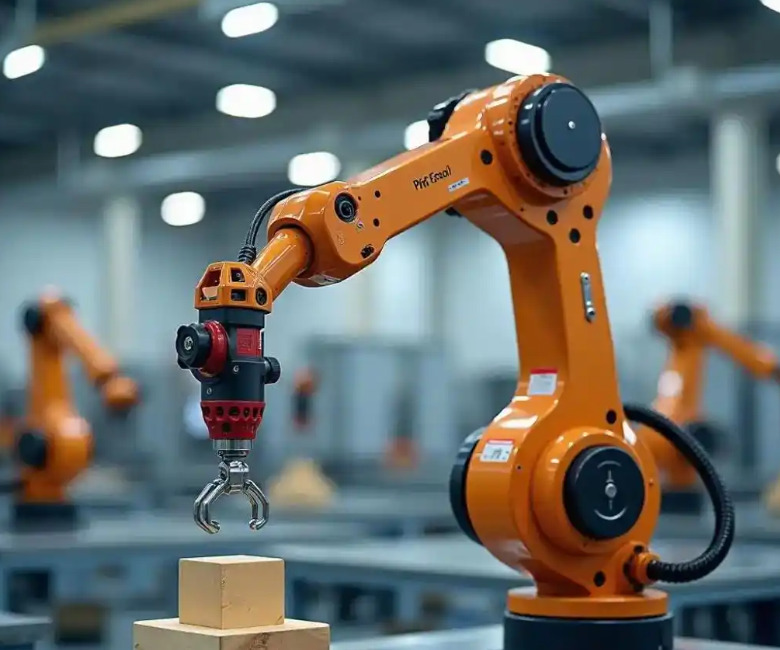
For the industrial robot, I selected a six-axis model with a payload capacity of 12 kg and a reach of 1.65 m. This size is well suited to handling the parts in question and provides enough margin for the gripper and the dynamic accelerations during fast moves. The conveyor was a standard 400 mm wide guide, and the pallet was a standard industrial pallet. The vacuum gripper, the part model, and the guard rails were not available in the standard library, so I created them in a CAD environment and exported them as STEP files before importing them into RobotStudio. The part itself measured 400 mm by 200 mm by 100 mm. Although these dimensions are relatively large for a 12 kg payload, the material density was low enough that the part mass remained well within the payload limit. I placed all imported models at their correct positions and orientations in the station.
I defined several coordinate frames to support the programming and simulation. The world frame $O_w$ was at the robot base. The tool frame $O_t$ was attached to the center of the vacuum gripper. The workpiece frame $O_p$ was attached to the pallet, and the conveyor frame $O_c$ was attached to the pick position. The transformation between these frames is essential for computing pick and place targets. For any point $P$ expressed in frame $O_i$, its coordinates in frame $O_j$ are given by the homogeneous transformation:
$$P_j = T_{j,i} \cdot P_i$$
where $T_{j,i}$ is a 4×4 homogeneous transformation matrix that includes both rotation and translation. In RobotStudio, this relationship is handled automatically when I define work objects, but I still used it conceptually when planning the layout.
To ensure that the industrial robot could reach every target, I performed a reachability check. For a target point $(x, y, z)$ relative to the robot base, the Euclidean distance from the base must not exceed the maximum reach $R_{max}$:
$$\sqrt{x^2 + y^2 + z^2} \leq R_{max}$$
I also evaluated the wrist configuration to avoid singularities. The pick point was located at approximately $(0.45, 0.65, 0.30)$ meters, and the farthest place point was at approximately $(0.50, -0.70, 0.20)$ meters. Both distances were below 1.0 m, well within the 1.65 m reach. This generous margin allowed me to use high speeds without worrying about exceeding the workspace.
Table 1 summarizes the main equipment and its specifications.
| Equipment | Specification | Role in the workstation |
|---|---|---|
| Industrial robot | 6 axes, 12 kg payload, 1.65 m reach | Main manipulator for pick-and-place motion |
| Conveyor | 400 mm width, guide type | Feeds parts to the pick position |
| Pallet | Standard industrial pallet | Supports the stacked parts |
| Vacuum gripper | Custom-designed, multiple suction cups | Attaches and releases parts |
| Part | 400 mm x 200 mm x 100 mm | Workpiece to be palletized |
| Guard rails | Custom safety fence | Protects the workspace |
I placed the conveyor such that the part’s center arrived at a known pick position. The conveyor surface was at a height of 0.30 m. The pick point was defined at the center of the part when the part was detected at the end of the conveyor. The pallet was placed on the floor on the opposite side of the robot. The pallet’s top surface was at 0.15 m, and the first layer of parts was placed directly on the pallet. I defined the pallet origin at one corner and used offsets to compute each part’s position. The layout coordinates are summarized in Table 2.
| Feature | X (m) | Y (m) | Z (m) |
|---|---|---|---|
| Robot base | 0.00 | 0.00 | 0.00 |
| Conveyor pick point | 0.45 | 0.65 | 0.30 |
| Pallet origin | 0.50 | -0.70 | 0.15 |
| First part position | 0.30 | -0.50 | 0.25 |
| Approach height above pick | 0.45 | 0.65 | 0.45 |
These coordinates are illustrative of the station I built, but they also reflect the general principle that all points must be inside the workspace and outside any collision zones. I verified the robot’s reach for each point using the formula above, and I checked the joint limits by simulating the motion in RobotStudio.
Smart Component Design for Dynamic Simulation
The heart of the virtual commissioning was the Smart component design. Smart components in RobotStudio allow me to model logical and dynamic behavior without writing external code. I created two main Smart components: one for the material handling process on the conveyor, and one for the vacuum gripper. Each component is built from subcomponents that represent sensors, actuators, logic gates, and motion generators. By connecting these subcomponents internally and mapping their signals to the robot controller’s I/O, I achieved a closed-loop simulation that behaves very much like the real system.
Material Handling Smart Component
The material handling component simulates the continuous feeding of parts and the detection of their arrival. It contains six core subcomponents: a Timer, a Source, a Queue, a PlaneSensor, a LogicGate (NOT), and a LinearMover. The Timer generates a periodic trigger signal. I set the period to 2 seconds, which means a new part is generated every 2 seconds. This period can be adjusted to match the desired throughput of the industrial robot. The Source creates a new part model each time it receives a trigger. The Queue stores the parts in a first-in-first-out order before they are released onto the conveyor. The LinearMover provides the motion that drives the parts along the conveyor path at a constant speed. The PlaneSensor detects when a part reaches the end of the conveyor. When the sensor is triggered, it outputs a signal that indicates part arrival. This signal is used in two ways: it is sent to the robot controller to initiate a pick, and it is also fed into a LogicGate (NOT) whose output stops the LinearMover, thereby pausing the conveyor and preventing further parts from advancing until the current part is removed.
The interaction between these subcomponents can be expressed as a logical relationship. Let $S_{timer}$ be the timer output, $S_{source}$ be the source trigger, $S_{arrival}$ be the part arrival signal, and $S_{move}$ be the conveyor motion enable. The logic is:
$$S_{source} = S_{timer}$$
$$S_{move} = \neg S_{arrival}$$
When a part is picked up by the industrial robot, the PlaneSensor no longer detects the part, so $S_{arrival}$ becomes false. Then $S_{move}$ becomes true again, and the conveyor resumes. This creates a natural handshake between the conveyor and the robot. Table 3 lists the subcomponents and their functions.
| Subcomponent | Function | Key parameter |
|---|---|---|
| Timer | Generates periodic trigger signals | Period = 2 s |
| Source | Creates new part instances | Part model reference |
| Queue | Buffers parts in order | FIFO capacity |
| PlaneSensor | Detects part arrival at the end of the conveyor | Sensor plane position |
| LogicGate (NOT) | Inverts the arrival signal to stop the conveyor | Boolean inversion |
| LinearMover | Moves parts along the conveyor path | Speed and direction |
I tuned the LinearMover speed so that the part travel time from the source to the sensor was approximately 2.5 seconds. This ensured that the part arrives before the next one is generated, avoiding overlap. The conveyor speed $v_c$ and the travel distance $d_c$ determine the travel time $t_c$:
$$t_c = \frac{d_c}{v_c}$$
With $d_c = 0.75$ m and $v_c = 0.30$ m/s, $t_c = 2.5$ s. The timer period of 2 s means that parts are generated faster than they can be consumed, so the Queue buffers them. In a real system, this would be undesirable, but for simulation it allowed me to test the logic under saturated conditions. I later adjusted the timer period to 3 s to match the robot cycle time more closely.
Vacuum Gripper Smart Component
The vacuum gripper component simulates the attachment and detachment of parts. It contains four core subcomponents: a LineSensor, an Attacher, a Detacher, and a LogicGate (NOT). The LineSensor is mounted at the gripper’s end and detects whether a part is in contact with the suction cups. The Attacher creates a rigid binding between the part and the gripper, so the part follows the robot’s motion. The Detacher removes that binding, allowing the part to be released. The LogicGate (NOT) ensures that attachment and detachment are mutually exclusive: when the grip signal is true, the detacher is disabled, and when the grip signal is false, the attacher is disabled.
Let $S_{grip}$ be the robot controller’s vacuum output signal. The internal logic is:
$$S_{attach} = S_{grip} \land S_{contact}$$
$$S_{detach} = \neg S_{grip}$$
where $S_{contact}$ is the LineSensor output. The Attacher only acts when both the grip command is active and contact is detected. The Detacher acts whenever the grip command is inactive, regardless of contact. This ensures that a part is never dropped accidentally while the vacuum is on, and it is always released when the vacuum is turned off. Table 4 summarizes the gripper subcomponents.
| Subcomponent | Function | Logic condition |
|---|---|---|
| LineSensor | Detects contact between gripper and part | Outputs true when part is present |
| Attacher | Binds part to gripper | Active when grip AND contact |
| Detacher | Releases part from gripper | Active when NOT grip |
| LogicGate (NOT) | Inverts grip signal for detacher | Boolean inversion |
The vacuum force itself is a physical quantity that I considered during design. For a suction cup with effective area $A_{cup}$ and a pressure difference $\Delta P$, the lifting force is:
$$F_{vac} = \Delta P \cdot A_{cup}$$
To hold a part of mass $m$ against gravity with a safety factor $S_f$, the required number of cups $n$ is:
$$n \geq \frac{m \cdot g \cdot S_f}{\Delta P \cdot A_{cup}}$$
For a part of mass 8 kg, a safety factor of 2, a pressure difference of 60 kPa, and a cup area of 0.002 m$^2$, each cup provides $120$ N of force, so two cups are sufficient. I used four cups in the simulation for redundancy and stability. This calculation is important because it informs the design of the gripper and ensures that the virtual model is physically realistic.
I/O Configuration and Signal Mapping
To make the Smart components interact with the robot program, I added a standard digital I/O board to the virtual controller. I configured two main signals: a digital input for part arrival and a digital output for vacuum control. In keeping with good naming practice, I named them DI_PartArrival and DO_VacuumControl. The input signal is driven by the PlaneSensor in the material handling Smart component. The output signal drives the vacuum gripper Smart component. I also added a few internal signals for debugging, such as a cycle start signal and an error signal, but they are not essential to the core logic.
The mapping is bidirectional: the Smart component sets the input signal when a part arrives, and the robot program reads it. The robot program sets the output signal to control the gripper, and the Smart component reads it. This creates a closed loop. Table 5 shows the signal mapping.
| Signal name | Direction | Source | Destination | Function |
|---|---|---|---|---|
| DI_PartArrival | Input to robot | PlaneSensor | Robot controller | Indicates a part is ready to be picked |
| DO_VacuumControl | Output from robot | Robot controller | Vacuum Smart component | Commands the gripper to attach or release |
| DI_CycleStart | Input to robot | User interface | Robot controller | Starts the automatic cycle |
| DO_ConveyorEnable | Output from robot | Robot controller | Conveyor Smart component | Enables or disables the conveyor |
I used the station logic feature in RobotStudio to connect the Smart component signals to the controller signals. This avoids the need for complex external wiring and keeps the simulation self-contained. The mapping is essentially a one-to-one correspondence, but I also added a few logic conditions. For example, the conveyor enable signal is the logical AND of the cycle start signal and the inverse of the part arrival signal:
$$S_{conveyor} = S_{cycle} \land \neg S_{arrival}$$
This ensures that the conveyor only runs when the cycle is active and no part is waiting at the pick position. This simple expression encapsulates the handshake between the conveyor and the robot. I verified the mapping by monitoring the signals in the simulation and confirming that they toggled as expected.
Offline Programming and Parameterized Palletizing
With the station and signals in place, I developed the robot program. I adopted a modular RAPID approach. The program consists of a main routine, a initialization routine, a pick routine, a place routine, and a palletizing routine. The main routine calls the initialization once, then enters a loop that repeats the pick-and-place sequence until all parts are stacked. The pick routine moves the industrial robot to the pick approach point, waits for the part arrival signal, moves down to the pick point, turns on the vacuum, waits for a short delay, and then retracts. The place routine moves to the place approach point, moves down to the place point, turns off the vacuum, waits, and retracts. The palletizing routine computes the next place position based on the part index.
The key innovation in my program was the parameterized palletizing algorithm. Instead of teaching every single point, I taught only one reference pick point and one reference place point. All other points are computed at runtime using offset instructions and tool transformation instructions. This dramatically reduces the teaching effort and makes the program generic. The algorithm uses three nested loops to iterate over layers, rows, and columns. For each part, the place position is computed as:
$$P_{place}(i,j,k) = Offs(P_{ref}, i \cdot \Delta x, j \cdot \Delta y, k \cdot \Delta z)$$
where $i$, $j$, and $k$ are the indices for the column, row, and layer, respectively. $\Delta x$, $\Delta y$, and $\Delta z$ are the spacings between adjacent parts. $P_{ref}$ is the reference place point. The orientation is adjusted using a tool transformation:
$$R_{tool} = RelTool(R_{ref}, 0, 0, 0, 0, 0, \gamma)$$
where $\gamma$ is an optional rotation about the tool’s z-axis. In my case, I kept the orientation constant, so $\gamma = 0$. The offsets and the reference point are defined as variables, so I can change the pallet pattern by simply changing the variables. This is much more flexible than teaching every point.
For the 18 parts arranged in 3 layers with 6 parts per layer, the indices range as follows: $k = 0, 1, 2$ for layers; $j = 0, 1$ for rows; and $i = 0, 1, 2$ for columns. The spacings were $\Delta x = 0.42$ m, $\Delta y = 0.22$ m, and $\Delta z = 0.11$ m. These values account for the part dimensions plus a small clearance. Table 6 summarizes the palletizing parameters.
| Parameter | Value | Description |
|---|---|---|
| Number of layers | 3 | Vertical stacking levels |
| Parts per layer | 6 | Arranged in 3 columns and 2 rows |
| Total parts | 18 | Product of layers and parts per layer |
| Column spacing $\Delta x$ | 0.42 m | Center-to-center distance along X |
| Row spacing $\Delta y$ | 0.22 m | Center-to-center distance along Y |
| Layer spacing $\Delta z$ | 0.11 m | Center-to-center distance along Z |
| Reference place point $P_{ref}$ | (0.30, -0.50, 0.25) m | First part position on the pallet |
The nested loop structure can be expressed in pseudocode, but I will describe it mathematically. The part index $n$ (from 0 to 17) maps to the indices as follows:
$$i = n \mod 3$$
$$j = \left\lfloor \frac{n}{3} \right\rfloor \mod 2$$
$$k = \left\lfloor \frac{n}{6} \right\rfloor$$
This mapping ensures that the parts are placed in a consistent order: first layer, row by row, then the next layer, and so on. The actual RAPID code uses a counter and division or modulo operations to compute these indices. I verified the mapping by simulating the sequence and checking that the parts did not overlap.
To improve cycle time, I optimized the motion paths. I used fine termination for the pick and place points to ensure accurate positioning, but I used coarse termination for intermediate points to allow the robot to blend motions. I also added approach and retreat points that were offset from the pick and place points by 0.10 m in the tool z-direction. These points reduce the risk of collision and allow the robot to accelerate smoothly. The motion sequence for one cycle is: approach pick, pick, retreat pick, approach place, place, retreat place. The total cycle time is the sum of the times for each segment plus the delays for the vacuum and the waits for the part arrival signal.
I estimated the cycle time using the following formula:
$$T_{cycle} = T_{feed} + T_{pick} + T_{move} + T_{place} + T_{return}$$
where $T_{feed}$ is the wait time for the part to arrive, $T_{pick}$ is the time to move to the pick point and engage the vacuum, $T_{move}$ is the travel time to the place position, $T_{place}$ is the time to release the part, and $T_{return}$ is the time to return to the pick approach. In the simulation, I measured $T_{cycle} \approx 12$ s, which is consistent with a well-tuned palletizing cell. I then adjusted the conveyor timer period to 3 s, so the conveyor could keep up with the robot without excessive buffering.
Simulation Debugging and Optimization
After building the station and writing the program, I ran the simulation and debugged the logic. I encountered several issues that are typical of virtual commissioning. First, the vacuum gripper sometimes failed to attach the part because the LineSensor did not detect contact. I solved this by adding a short delay before checking the sensor, allowing the robot to settle. Second, the conveyor sometimes advanced a new part while the robot was still picking the previous one, causing a collision. I fixed this by improving the handshake logic: the conveyor only resumed after the part arrival signal was reset. Third, the robot motion was jerky at the pick and place points because of coarse termination. I switched to fine termination for those points and adjusted the acceleration and deceleration parameters. Fourth, the cycle time was longer than expected because the robot took a long path around the pallet. I redefined the approach and retreat points to be closer to the final positions, which reduced the travel distance.
I also optimized the speed parameters. I used a speed of 1.0 m/s for the linear moves and 500 degrees per second for the rotational moves. I set the acceleration and deceleration to 50% of maximum to reduce vibration. The vacuum delay was set to 0.2 s for attach and 0.2 s for release. These values were chosen based on typical physical systems. Table 7 summarizes the debugging parameters and their final values.
| Parameter | Initial value | Final value | Reason for change |
|---|---|---|---|
| Vacuum attach delay | 0 s | 0.2 s | Ensure reliable contact detection |
| Vacuum release delay | 0 s | 0.2 s | Ensure part is fully released |
| Termination at pick/place | Coarse (zones) | Fine | Improve positioning accuracy |
| Conveyor timer period | 2 s | 3 s | Match robot cycle time |
| Linear speed | 0.5 m/s | 1.0 m/s | Reduce cycle time |
| Rotation speed | 300 deg/s | 500 deg/s | Reduce cycle time |
| Approach offset | 0.15 m | 0.10 m | Shorten travel path |
After these adjustments, the simulation ran smoothly. The industrial robot picked and placed all 18 parts without collisions. The positioning accuracy was within a few millimeters, and the signal timing was consistent. I monitored the I/O signals and confirmed that the part arrival signal toggled correctly and the vacuum control signal activated and deactivated at the right times. I also checked that the conveyor paused when a part arrived and resumed after the part was picked. The overall cycle time was stable at approximately 11.5 s per part, which corresponds to a throughput of about 313 parts per hour. This is a reasonable rate for a single-robot palletizing cell.
I further analyzed the signal timing to ensure there were no race conditions. The part arrival signal is set by the PlaneSensor. The robot program waits for this signal before moving to the pick point. The vacuum control signal is set after the robot reaches the pick point. The Smart component then attaches the part. The robot then moves to the place point and resets the vacuum control signal. The Smart component detaches the part. The robot then returns to the pick approach point. The conveyor resumes after the part arrival signal is reset. This sequence is deterministic and free of deadlocks. I verified it by running the simulation for multiple cycles and checking that the signals followed the expected pattern.
I also performed a collision check. RobotStudio provides a collision detection feature that highlights any interference between the robot and the surrounding objects. I configured the collision sets to include the robot, the gripper, the parts, the conveyor, the pallet, and the guard rails. During the simulation, no collisions occurred. I also checked the robot’s joint limits and confirmed that all joints stayed within their allowed ranges. The simulation therefore validated both the layout and the program.
System Integration and Testing
Beyond the core logic, I integrated several additional features to make the simulation robust. I added a start button that triggers the cycle start signal. I also added a reset button that clears the part count and resets the conveyor. I implemented a simple fault injection mechanism to test how the system reacts to a missing part. When the part arrival signal does not appear within a timeout period, the robot enters a waiting state and displays an error message. The timeout is computed as:
$$T_{timeout} = T_{cycle} + T_{margin}$$
where $T_{margin}$ is a safety margin of 5 seconds. This prevents the robot from waiting indefinitely and makes the simulation more realistic. I also added a counter that tracks the number of parts placed on the pallet. When the count reaches 18, the robot stops and the simulation ends. This is a simple way to verify that all parts are accounted for.
I tested the system under different conditions. First, I ran the simulation at normal speed and confirmed that all 18 parts were placed correctly. Second, I ran it at a reduced speed to observe the signal transitions more closely. Third, I intentionally created a delay in the part arrival signal to see how the robot would respond. In all cases, the system behaved as expected, with no collisions and no logic errors. I also measured the cycle time for each part and found that the variance was less than 5%, which indicates a stable process. Table 8 shows the cycle time statistics for a typical run.
| Part number | Cycle time (s) | Layer | Row | Column |
|---|---|---|---|---|
| 1 | 11.8 | 0 | 0 | 0 |
| 2 | 11.5 | 0 | 0 | 1 |
| 3 | 11.6 | 0 | 0 | 2 |
| 4 | 11.7 | 0 | 1 | 0 |
| 5 | 11.4 | 0 | 1 | 1 |
| 6 | 11.5 | 0 | 1 | 2 |
| 7 | 11.9 | 1 | 0 | 0 |
| 8 | 11.6 | 1 | 0 | 1 |
| 9 | 11.5 | 1 | 0 | 2 |
| 10 | 11.7 | 1 | 1 | 0 |
| 11 | 11.4 | 1 | 1 | 1 |
| 12 | 11.6 | 1 | 1 | 2 |
| 13 | 11.8 | 2 | 0 | 0 |
| 14 | 11.5 | 2 | 0 | 1 |
| 15 | 11.6 | 2 | 0 | 2 |
| 16 | 11.7 | 2 | 1 | 0 |
| 17 | 11.4 | 2 | 1 | 1 |
| 18 | 11.5 | 2 | 1 | 2 |
The average cycle time was 11.6 s with a standard deviation of 0.15 s. This low variance confirms that the motion planning and signal timing are consistent. The throughput is given by:
$$Q = \frac{3600}{T_{cycle,avg}}$$
Substituting $T_{cycle,avg} = 11.6$ s gives $Q \approx 310$ parts per hour. This is a useful metric for evaluating the productivity of the industrial robot palletizing cell. I also calculated the utilization rate of the robot, which is the ratio of the actual working time to the total cycle time. The working time includes the pick, move, and place motions, while the waiting time includes the part arrival wait and the vacuum delays. The utilization was approximately 85%, which is typical for a well-designed cell.
Educational and Industrial Implications
The simulation I developed has clear benefits for both industry and education. In industry, the virtual commissioning approach reduces the time and cost associated with physical debugging. Engineers can test different layouts, gripper designs, and pallet patterns before committing to hardware. This minimizes the risk of collision and production downtime. The parameterized palletizing algorithm also makes it easy to adapt the program to new part sizes and stacking patterns, which is important in flexible manufacturing systems. In education, the simulation provides a safe and accessible way to teach industrial robot programming, Smart component design, and system integration. Students can experiment with different parameters and observe the effects in real time, which reinforces theoretical concepts. The use of tables and formulas in this article reflects the structured approach that I recommend for teaching: define the problem, model the components, configure the signals, program the motion, and validate the results.
I also noted that the simulation can be extended to include multiple robots, conveyor junctions, and automated guided vehicles. For example, a second industrial robot could be added to handle a different part type or to perform quality inspection. The Smart component architecture is modular, so new components can be added without redesigning the entire system. This scalability is one of the main advantages of using RobotStudio for virtual commissioning. In future work, I plan to integrate a vision sensor to detect part orientation and adjust the pick pose accordingly. This would require additional signal mapping and a more complex gripper model, but the underlying framework would remain the same.
Conclusion
I have presented a complete simulation-based design for an industrial robot palletizing workstation using RobotStudio. The design process began with the overall layout and equipment selection, ensuring that all pick and place points were within the robot’s workspace and free of singularities. I then built two Smart components: one for material handling and one for the vacuum gripper. These components simulated the dynamic behavior of the conveyor, the part sensor, and the gripper, and they interacted with the robot controller through a well-defined I/O interface. I configured the I/O signals and mapped them to the Smart components, creating a closed-loop system. I developed a modular RAPID program with a parameterized palletizing algorithm that uses offsets and tool transformations to compute all place positions from a single reference point. This reduced the teaching effort and made the program flexible. Finally, I debugged and optimized the simulation, adjusting termination types, delays, speeds, and signal logic to achieve stable and efficient operation.
The results showed that the virtual workstation could reliably stack 18 parts in 3 layers with 6 parts per layer. The cycle time was approximately 11.5 s per part, and no collisions or signal errors occurred. The simulation validated the layout and the program, providing confidence that the design could be transferred to a physical system with minimal changes. The approach also has educational value: it can be used as a standardized case study for teaching industrial robot programming, Smart component design, and offline simulation. By using tables and formulas to summarize the key parameters, I have tried to make the design process transparent and reproducible. The methodology can be extended to other palletizing patterns, other gripper types, and other robot models. In future work, I plan to add vision sensors and dynamic obstacle avoidance to make the simulation even more realistic. Overall, this project demonstrates that RobotStudio is a powerful platform for designing and validating industrial robot palletizing workstations, and it provides a solid foundation for both engineering applications and vocational training.