
I focus on the absolute positioning accuracy of industrial robots because it directly determines the quality of high-precision tasks such as welding, grinding, drilling, and assembly. In my work, I treat the end-effector pose error of industrial robots as a superposition of two physically distinct components: geometric error caused by manufacturing and assembly deviations, and flexibility-induced error caused by payload variation and joint compliance. I develop a dual-branch physics-informed neural network with an adaptive constraint weight adapter, which I call PC-DBPINN-CWA. The proposed method is designed to predict both geometric and flexibility errors of industrial robots under variable payload conditions and to support online feedforward compensation. I validate the method on a six-degree-of-freedom industrial robot and compare it with several purely data-driven and parametric approaches.
1. Introduction
Industrial robots are widely used in modern manufacturing. However, their absolute positioning accuracy is often inferior to their repeatability. In my experiments and analysis, I observe that the pose error of industrial robots arises from at least two major sources. The first source is geometric error, which is introduced by link parameter deviations, joint zero offsets, and assembly imperfections. The second source is flexibility error, which is induced by payload changes and elastic deformation of joints and links. Because the two error sources have different physical mechanisms, I argue that they should not be modeled by a single black-box mapping. Instead, I separate them into two parallel branches and embed physical constraints into each branch.
Parametric calibration methods, such as those based on the modified Denavit-Hartenberg model, the product of exponentials, and conformal geometric algebra, can identify geometric parameters. However, they usually require a complete mathematical model and cannot easily compensate for payload-dependent flexibility errors. Non-parametric methods, including support vector regression, Gaussian process regression, and various neural networks, can learn a direct mapping from joint angles or theoretical poses to pose errors. Nevertheless, these methods often suffer from poor interpretability and limited extrapolation capability when the payload changes. I therefore propose a physics-constrained dual-branch framework that preserves data-driven learning while enforcing physical consistency.
My main contributions are as follows. First, I construct a dual-branch physics-informed neural network for industrial robots. The geometric branch uses the theoretical end-effector pose as input, and the flexibility branch uses payload mass, center-of-mass position, joint velocity, and joint acceleration as inputs. Second, I embed geometric smoothness, force-deformation direction consistency, and energy conservation constraints into the loss function. Third, I design a residual-feedback adaptive constraint weight scheduling mechanism to balance data fidelity and physical constraints during training. Fourth, I conduct extensive experiments on a KUKA KR16-2 industrial robot under multiple payload conditions and demonstrate that the proposed method improves both prediction accuracy and online compensation performance.
2. Kinematic and Error Modeling of Industrial Robots
I model the pose error of industrial robots as the sum of a geometric component and a flexibility component. Under the assumption of small deformation and quasi-static operation, the total pose error can be written as
$$ \delta e = \delta e_g + \delta e_f $$
where \(\delta e_g\) denotes the geometric error and \(\delta e_f\) denotes the flexibility error. I use a six-dimensional vector to represent each component:
$$ \delta e_g = \begin{bmatrix} \delta X_g & \delta Y_g & \delta Z_g & \delta A_g & \delta B_g & \delta C_g \end{bmatrix}^T $$
$$ \delta e_f = \begin{bmatrix} \delta X_f & \delta Y_f & \delta Z_f & \delta A_f & \delta B_f & \delta C_f \end{bmatrix}^T $$
Here, \(X\), \(Y\), and \(Z\) are the position coordinates, while \(A\), \(B\), and \(C\) are the orientation angles. I use the modified Denavit-Hartenberg convention to build the forward kinematics of the industrial robot.
2.1 Forward Kinematics
The transformation between adjacent joint frames is expressed as
$$ {}^{i-1}T_i = Rot(\theta_i) Trans(d_i) Trans(a_i) Rot(\alpha_i) Rot(\beta_i) $$
where \(\theta_i\) is the joint angle, \(d_i\) is the link offset, \(a_i\) is the link length, \(\alpha_i\) is the link twist, and \(\beta_i\) is an additional rotation about the \(Y\)-axis used for adjacent parallel joints. The end-effector pose relative to the base frame is obtained by multiplying the individual transformation matrices:
$$ {}^{0}T_6 = {}^{0}T_1 {}^{1}T_2 {}^{2}T_3 {}^{3}T_4 {}^{4}T_5 {}^{5}T_6 = \begin{bmatrix} R & P \\ 0 & 1 \end{bmatrix} $$
where \(R\) is the orientation matrix and \(P = [X, Y, Z]^T\) is the position vector. I convert the orientation matrix to Euler angles using
$$ A = \arctan 2(r_{32}, r_{33}) $$
$$ B = \arctan 2(-r_{31}, \sqrt{r_{11}^2 + r_{21}^2}) $$
$$ C = \arctan 2(r_{21}, r_{11}) $$
Table 1 lists the kinematic parameters I use for the industrial robot in my study.
| Joint | \(a_i\) / mm | \(\alpha_i\) / deg | \(d_i\) / mm | \(\theta_i\) / deg | \(\beta_i\) / deg |
|---|---|---|---|---|---|
| 1 | 0 | 0 | 675 | \(\theta_1\) | 0 |
| 2 | 260 | -90 | 0 | \(-90 + \theta_2\) | \(\beta_2\) |
| 3 | 680 | 0 | 0 | \(\theta_3\) | 0 |
| 4 | -35 | -90 | 670 | \(\theta_4\) | 0 |
| 5 | 0 | 90 | 0 | \(\theta_5\) | 0 |
| 6 | 0 | -90 | 158 | \(180 + \theta_6\) | 0 |
2.2 Geometric Error of Industrial Robots
Geometric error in industrial robots originates from deviations in the kinematic parameters. Let the theoretical parameters be \(\theta_i, d_i, a_i, \alpha_i, \beta_i\), and let the actual parameters be \(\theta_i + \Delta \theta_i\), \(d_i + \Delta d_i\), \(a_i + \Delta a_i\), \(\alpha_i + \Delta \alpha_i\), and \(\beta_i + \Delta \beta_i\). The transformation matrix with geometric errors is denoted by \(T_g\). The geometric error matrix is then
$$ \delta T = T_g – T_0 $$
where \(T_0\) is the nominal transformation matrix. The geometric pose error vector is
$$ \delta e_g = \begin{bmatrix} \delta X_g & \delta Y_g & \delta Z_g & \delta A_g & \delta B_g & \delta C_g \end{bmatrix}^T $$
I model the geometric error as a smooth function of the robot configuration. In my dual-branch network, the geometric branch takes the theoretical pose as input and predicts \(\delta e_g\). Because geometric error is caused by fixed structural deviations, it should vary smoothly with joint angles. I enforce this property by adding a geometric smoothness constraint to the loss function.
2.3 Flexibility Error of Industrial Robots
Flexibility error of industrial robots is caused by elastic deformation under payload. I consider the payload mass, payload center of mass, joint velocity, and joint acceleration. The joint torque under external load is
$$ \tau(\theta) = J^T(\theta) F $$
where \(J(\theta)\) is the Jacobian matrix and \(F\) is the external force/torque vector at the end effector. I approximate each joint as a linear torsional spring, so the elastic deformation is
$$ \Delta \theta = C \tau(\theta) $$
where \(C\) is the joint compliance matrix given by
$$ C = \begin{bmatrix} c_1 & 0 & \cdots & 0 \\ 0 & c_2 & \cdots & 0 \\ \vdots & \vdots & \ddots & \vdots \\ 0 & 0 & \cdots & c_6 \end{bmatrix} $$
The flexibility-induced end-effector error is mapped through the differential kinematics:
$$ \delta e_f = J(\theta) \Delta \theta $$
Substituting the torque and compliance expressions gives
$$ \delta e_f = J(\theta) C J^T(\theta) F $$
Table 2 lists the joint compliance coefficients I use for the industrial robot.
| Joint | 1 | 2 | 3 | 4 | 5 | 6 |
|---|---|---|---|---|---|---|
| Compliance coefficient / (rad/(N·mm)) | \(4.0 \times 10^{-9}\) | \(2.9 \times 10^{-9}\) | \(5.6 \times 10^{-9}\) | \(1.4 \times 10^{-8}\) | \(4.5 \times 10^{-8}\) | \(2.3 \times 10^{-7}\) |
The flexibility branch in my network uses the payload mass \(m\), the payload center of mass \([x_{cog}, y_{cog}, z_{cog}]^T\), the mean absolute joint velocity \(\bar{q}\), and the mean absolute joint acceleration \(\bar{\ddot{q}}\) as inputs. I reconstruct the velocity and acceleration using central difference:
$$ \dot{q}_i(t_k) \approx \frac{q_i(t_{k+1}) – q_i(t_{k-1})}{2 \Delta t} $$
$$ \ddot{q}_i(t_k) \approx \frac{q_i(t_{k+1}) – 2 q_i(t_k) + q_i(t_{k-1})}{\Delta t^2} $$
I then compute the mean values over all six joints:
$$ \bar{q} = \frac{1}{6} \sum_{i=1}^{6} |\dot{q}_i| $$
$$ \bar{\ddot{q}} = \frac{1}{6} \sum_{i=1}^{6} |\ddot{q}_i| $$
Thus, the input vector of the flexibility branch is
$$ x_f = \begin{bmatrix} x_{cog} & y_{cog} & z_{cog} & m & \bar{q} & \bar{\ddot{q}} \end{bmatrix}^T $$
3. Physics-Constrained Dual-Branch PINN for Industrial Robots
I use a physics-informed neural network to model the error of industrial robots because it can combine measurement data with physical laws. A standard PINN loss consists of a data term and a physics term:
$$ L_{total} = L_{data} + L_{ph} $$
The data loss is
$$ L_{data} = \frac{1}{N} \sum_{n=1}^{N} \left\| \hat{y}^{(n)} – y^{(n)} \right\|_2^2 $$
where \(\hat{y}^{(n)}\) is the predicted error vector and \(y^{(n)}\) is the measured error vector. In my dual-branch architecture, I separate the prediction into a geometric branch \(g\) and a flexibility branch \(f\):
$$ \hat{e}_g = \mathcal{N}_g(x_g; \xi_g) $$
$$ \hat{e}_f = \mathcal{N}_f(x_f; \xi_f) $$
The total predicted pose error is
$$ \hat{e} = \hat{e}_g + \hat{e}_f $$
The geometric branch input is the theoretical pose:
$$ x_g = \begin{bmatrix} X & Y & Z & A & B & C \end{bmatrix}^T $$
The flexibility branch input is the payload and motion state vector defined in Section 2.3. Both branches are fully connected networks with rectified linear unit activations. I use three hidden layers for each branch in my implementation.
3.1 Geometric Smoothness Constraint
Geometric error of industrial robots should vary smoothly with joint angles. I enforce this by penalizing the gradient of the predicted geometric error with respect to joint angles:
$$ L_{geo} = \frac{1}{N} \sum_{n=1}^{N} \sum_{i=1}^{6} \left\| \frac{\partial \hat{e}_g^{(n)}}{\partial \theta_i} \right\|_2^2 $$
This constraint suppresses non-physical oscillations and encourages the network to learn a smooth geometric error field.
3.2 Force-Deformation Direction Consistency Constraint
For the flexibility branch, I require the predicted deformation direction to be consistent with the theoretical deformation direction. The theoretical deformation under an external force is
$$ d_{theory} = C_{cart}(\theta) F $$
The Cartesian compliance matrix is
$$ C_{cart}(\theta) = J(\theta) C J^T(\theta) $$
The predicted deformation direction is
$$ d_{pred} = \frac{\hat{p}_f}{\|\hat{p}_f\|} $$
where \(\hat{p}_f = [\delta \hat{X}_f, \delta \hat{Y}_f, \delta \hat{Z}_f]^T\) is the predicted position deformation. The direction consistency loss is
$$ L_{direction} = \frac{1}{N} \sum_{n=1}^{N} \left( 1 – d_{pred}^{(n)} \cdot d_{theory}^{(n)} \right)^2 $$
This term encourages the predicted deformation to align with the direction dictated by the stiffness of the industrial robot.
3.3 Energy Conservation Constraint
I also impose an energy conservation constraint. The external work done by the payload gravity on the flexible deformation should equal the strain energy stored in the structure:
$$ W_{external} = U_{strain} $$
The external work is approximated as
$$ W_{external} = G \cdot p_f $$
where \(G\) is the gravitational force vector and \(p_f\) is the deformation vector. The strain energy is
$$ U_{strain} = \frac{1}{2} k \|p_f\|^2 $$
with the equivalent stiffness coefficient
$$ k = \frac{1}{J(\theta) C J^T(\theta)} $$
The energy conservation loss is
$$ L_{energy} = \frac{1}{N} \sum_{n=1}^{N} \left| W_{external}^{(n)} – U_{strain}^{(n)} \right| $$
This constraint prevents the predicted deformation from violating the global energy balance of the industrial robot.
3.4 Branch Loss Functions
The geometric branch loss is
$$ L_g = \lambda_{g,1} L_{data}^g + \lambda_{g,2} L_{geo} $$
The flexibility branch loss is
$$ L_f = \lambda_{f,1} L_{data}^f + \lambda_{f,2} L_{direction} + \lambda_{f,3} L_{energy} $$
where \(\lambda\) are weighting coefficients. Instead of fixing these weights manually, I use an adaptive constraint weight adapter.
4. Adaptive Constraint Weight Adapter
Different loss terms in a physics-informed neural network have different scales and convergence behaviors. Fixed weights can cause training instability or imbalance between data fitting and physical consistency. I therefore introduce an uncertainty-based adaptive weighting mechanism. For each loss term \(a\), I introduce a learnable parameter \(\sigma_a\) and write the weighted loss as
$$ L_{CWA} = \sum_a \left( \frac{1}{2 \sigma_a^2} L_a + \log \sigma_a \right) $$
The effective weight of loss term \(a\) is
$$ \lambda_a = \frac{1}{2 \sigma_a^2} $$
When a constraint has a large residual, \(\sigma_a\) increases and the corresponding weight decreases. When the residual becomes small and stable, \(\sigma_a\) decreases and the physical constraint receives more weight. The logarithmic term prevents \(\sigma_a\) from diverging. I apply this adapter to both the geometric branch and the flexibility branch. In my experiments, I observe that the data loss weight decreases during training while the physical constraint weights increase, which indicates that the industrial robot model gradually shifts from data-driven fitting to physics-consistent prediction.
| Branch | Constraint | Physical meaning | Mathematical form |
|---|---|---|---|
| Geometric | Geometric smoothness | Geometric error of industrial robots varies smoothly with joint angles | \(L_{geo} = \frac{1}{N} \sum \sum_i \| \partial \hat{e}_g / \partial \theta_i \|^2\) |
| Flexibility | Force-deformation direction consistency | Deformation direction follows the Cartesian stiffness of industrial robots | \(L_{direction} = \frac{1}{N} \sum (1 – d_{pred} \cdot d_{theory})^2\) |
| Flexibility | Energy conservation | External work equals strain energy in elastic deformation | \(L_{energy} = \frac{1}{N} \sum | W_{external} – U_{strain} |\) |
5. Experimental Setup and Data Collection
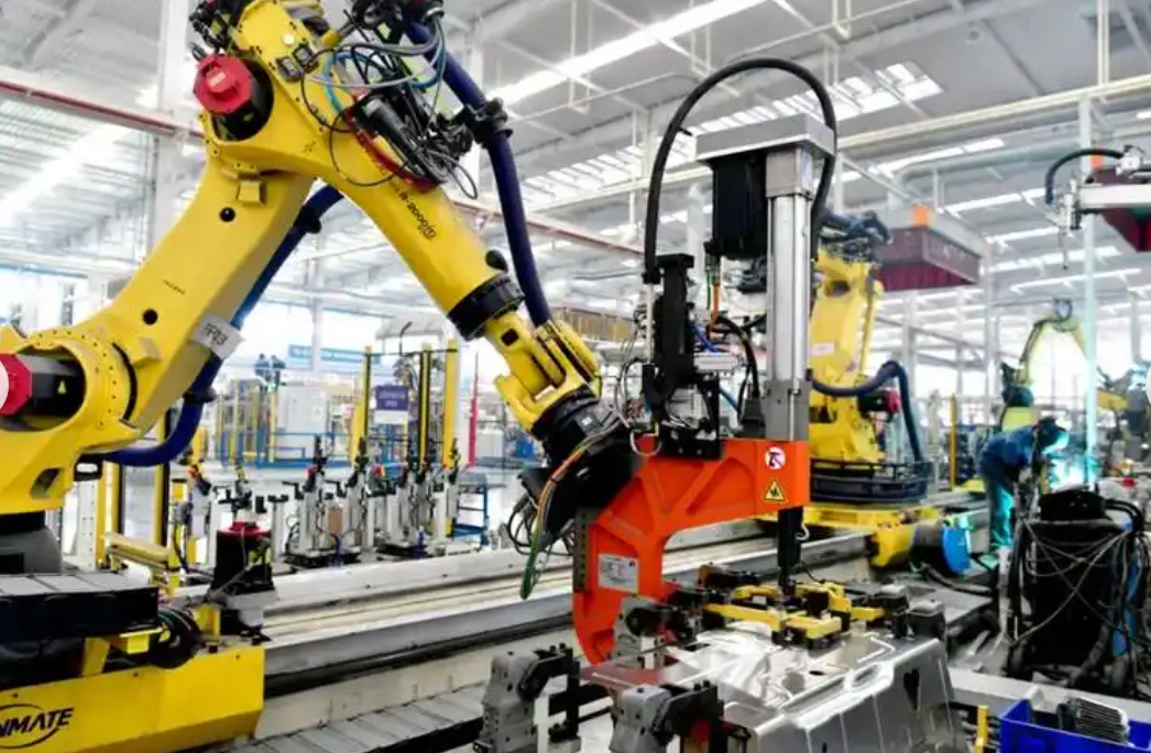
I built an experimental platform with a six-axis industrial robot, a laser tracker, and a target mounted on the end effector. The laser tracker measures the end-effector pose with high accuracy. I developed an online communication and control software that sends motion commands to the robot controller through TCP/IP and acquires theoretical pose and joint angle data. The experimental configuration is shown below.
I selected four payload conditions within the rated payload of the industrial robot: no payload, 7 kg, 11 kg, and 15 kg. I also used three unseen payloads of 4.6 kg, 8.6 kg, and 12.6 kg for online compensation validation. The measurement volume was a cube with a side length of 500 mm, and I divided it into a spatial grid with 50 mm spacing. This produced 1331 measurement points per payload condition. I collected 5324 points in total and split them into training and validation sets at a ratio of 8:2. During data collection, the industrial robot moved at 50% of its rated speed. Table 4 summarizes the payload conditions and data usage.
| Payload condition | Mass / kg | Number of points | Purpose |
|---|---|---|---|
| No payload | 0 | 1331 | Geometric error learning |
| Payload 1 | 7 | 1331 | Flexibility error learning |
| Payload 2 | 11 | 1331 | Flexibility error learning |
| Payload 3 | 15 | 1331 | Flexibility error learning |
| Unseen payload A | 4.6 | 20 | Online compensation validation |
| Unseen payload B | 8.6 | 20 | Online compensation validation |
| Unseen payload C | 12.6 | 20 | Online compensation validation |
I observed that the position error of industrial robots increases with payload. In the no-load condition, the mean absolute position error was about 0.308 mm. Under the 15 kg payload, the mean absolute error increased to about 0.889 mm, and the maximum absolute error reached about 1.457 mm. The Z-direction error showed a clear negative shift due to gravity-induced deformation. The X-direction error also shifted, while the Y-direction error remained centered near zero but with larger dispersion. These observations confirm that payload variation strongly affects the flexibility error of industrial robots.
6. Ablation Study
I conducted an ablation study to evaluate the contribution of each component in my proposed model. I compared the following configurations: a single-branch PINN, a dual-branch PINN without physical constraints, a dual-branch PINN with only geometric smoothness, a dual-branch PINN with only direction consistency, a dual-branch PINN with only energy conservation, a dual-branch PINN with all constraints but fixed weights, and the full PC-DBPINN-CWA model. The root mean square error of position and orientation was used as the evaluation metric. Table 5 presents the ablation results.
| Model | Payload | Position RMSE / mm | Orientation RMSE / deg |
|---|---|---|---|
| PINN | No load | 0.08009 | 0.06585 |
| PINN | 7 kg | 0.24126 | 0.12321 |
| PINN | 11 kg | 0.31173 | 0.13710 |
| PINN | 15 kg | 0.38162 | 0.14859 |
| DBPINN | No load | 0.07407 | 0.05278 |
| DBPINN | 7 kg | 0.20301 | 0.09957 |
| DBPINN | 11 kg | 0.27946 | 0.11058 |
| DBPINN | 15 kg | 0.36128 | 0.12087 |
| PC-DBPINN + geo | No load | 0.05821 | 0.04512 |
| PC-DBPINN + geo | 7 kg | 0.18235 | 0.09345 |
| PC-DBPINN + geo | 11 kg | 0.27185 | 0.11876 |
| PC-DBPINN + geo | 15 kg | 0.34267 | 0.12984 |
| PC-DBPINN + direction | No load | 0.06412 | 0.04893 |
| PC-DBPINN + direction | 7 kg | 0.17025 | 0.08537 |
| PC-DBPINN + direction | 11 kg | 0.23874 | 0.10625 |
| PC-DBPINN + direction | 15 kg | 0.29816 | 0.10842 |
| PC-DBPINN + energy | No load | 0.06685 | 0.05021 |
| PC-DBPINN + energy | 7 kg | 0.17654 | 0.08972 |
| PC-DBPINN + energy | 11 kg | 0.23147 | 0.09854 |
| PC-DBPINN + energy | 15 kg | 0.27639 | 0.10411 |
| PC-DBPINN + all fixed | No load | 0.06267 | 0.04634 |
| PC-DBPINN + all fixed | 7 kg | 0.19266 | 0.09167 |
| PC-DBPINN + all fixed | 11 kg | 0.24768 | 0.11034 |
| PC-DBPINN + all fixed | 15 kg | 0.30647 | 0.11091 |
| PC-DBPINN-CWA | No load | 0.05339 | 0.04390 |
| PC-DBPINN-CWA | 7 kg | 0.16084 | 0.08214 |
| PC-DBPINN-CWA | 11 kg | 0.20782 | 0.09133 |
| PC-DBPINN-CWA | 15 kg | 0.25441 | 0.09687 |
The ablation results show that the dual-branch structure improves prediction accuracy compared with a single-branch PINN. Under the 15 kg payload, the position RMSE decreases from 0.38162 mm to 0.36128 mm, and the orientation RMSE decreases from 0.14859° to 0.12087°. When I add physical constraints, the error decreases further. The geometric smoothness constraint is most effective in the no-load condition, which confirms that it captures the smooth variation of geometric error. The direction consistency constraint improves performance under medium and high payloads, and the energy conservation constraint is particularly effective at suppressing error divergence under heavy payloads. When all constraints are used with fixed weights, the position RMSE under 11 kg is 0.24768 mm, which is lower than the unconstrained dual-branch model. The full PC-DBPINN-CWA model achieves the best performance in all cases. Under 15 kg, the position RMSE is 0.25441 mm and the orientation RMSE is 0.09687°. Compared with the single-branch PINN, the position RMSE is reduced by about 33.33% and the orientation RMSE by about 34.81%.
7. Comparison with Other Methods
I compared my method with three existing error prediction methods. I used the same training and validation data for all methods. The evaluation metrics include RMSE, mean absolute error, and maximum absolute error for both position and orientation. Table 6 summarizes the comparison under four payload conditions.
| Method | Payload | Position RMSE / mm | Position MAE / mm | Position Max / mm | Orientation RMSE / deg | Orientation MAE / deg | Orientation Max / deg |
|---|---|---|---|---|---|---|---|
| Method A | No load | 0.06184 | 0.04912 | 0.17047 | 0.04976 | 0.03984 | 0.11372 |
| Method A | 7 kg | 0.17896 | 0.14258 | 0.46328 | 0.09238 | 0.07394 | 0.21285 |
| Method A | 11 kg | 0.22874 | 0.18273 | 0.60319 | 0.10284 | 0.08236 | 0.23617 |
| Method A | 15 kg | 0.28291 | 0.22546 | 0.73928 | 0.11063 | 0.08858 | 0.25394 |
| Method B | No load | 0.06792 | 0.05416 | 0.18235 | 0.05572 | 0.04458 | 0.12836 |
| Method B | 7 kg | 0.19453 | 0.15527 | 0.50834 | 0.10142 | 0.08116 | 0.23348 |
| Method B | 11 kg | 0.25164 | 0.20131 | 0.65842 | 0.11347 | 0.09076 | 0.25934 |
| Method B | 15 kg | 0.30946 | 0.24738 | 0.80716 | 0.12385 | 0.09908 | 0.28615 |
| Method C | No load | 0.07325 | 0.05843 | 0.19456 | 0.05984 | 0.04786 | 0.13745 |
| Method C | 7 kg | 0.20837 | 0.16642 | 0.54681 | 0.10853 | 0.08674 | 0.24836 |
| Method C | 11 kg | 0.27184 | 0.21735 | 0.71248 | 0.12184 | 0.09742 | 0.28153 |
| Method C | 15 kg | 0.33218 | 0.26576 | 0.86935 | 0.13246 | 0.10596 | 0.30642 |
| My method | No load | 0.05339 | 0.04163 | 0.16352 | 0.04390 | 0.03512 | 0.10184 |
| My method | 7 kg | 0.16084 | 0.12794 | 0.42386 | 0.08214 | 0.06571 | 0.19452 |
| My method | 11 kg | 0.20782 | 0.16573 | 0.54892 | 0.09133 | 0.07306 | 0.21637 |
| My method | 15 kg | 0.25441 | 0.20286 | 0.68247 | 0.09687 | 0.07749 | 0.22964 |
My method achieves the lowest RMSE, MAE, and maximum error in all payload conditions. For position prediction under 15 kg, the RMSE is 0.25441 mm, which is about 10.08% lower than the best competing method. The orientation RMSE under 15 kg is 0.09687°, which is about 12.44% lower than the best competing method. The improvement is more pronounced under heavy payloads, which confirms that the physics constraints and the dual-branch design improve the extrapolation ability of the model for industrial robots.
8. Online Compensation and Validation
I implement online feedforward compensation based on the predicted pose error. The compensation flow is as follows. First, the proposed model predicts the geometric error and the flexibility error for a target pose and payload condition. Second, the two error components are fused to obtain the total pose error. Third, the total error is negated and sent to the robot controller through TCP/IP. Fourth, the controller adjusts the motion command online. The inference time of my model is about 8.983 ms, which satisfies the real-time requirement for online compensation of industrial robots.
The compensation command is
$$ u_{comp} = – \hat{e} = – ( \hat{e}_g + \hat{e}_f ) $$
I validate the compensation on three unseen payloads: 4.6 kg, 8.6 kg, and 12.6 kg. I select 20 validation points along diagonal trajectories that cover the main workspace of the industrial robot. These points are not used in training. Table 7 lists the compensation results.
| Payload | Method | Position Max / mm | Position MAE / mm | Position STD / mm | Orientation Max / deg | Orientation MAE / deg | Orientation STD / deg |
|---|---|---|---|---|---|---|---|
| 4.6 kg | Before compensation | 0.794 | 0.358 | 0.199 | 0.871 | 0.345 | 0.261 |
| 4.6 kg | My method | 0.207 | 0.101 | 0.052 | 0.249 | 0.112 | 0.062 |
| 4.6 kg | Parametric method | 0.271 | 0.126 | 0.071 | 0.244 | 0.109 | 0.060 |
| 4.6 kg | Non-parametric method | 0.335 | 0.112 | 0.070 | 0.360 | 0.147 | 0.090 |
| 8.6 kg | Before compensation | 1.171 | 0.506 | 0.265 | 0.920 | 0.431 | 0.215 |
| 8.6 kg | My method | 0.345 | 0.155 | 0.078 | 0.270 | 0.178 | 0.041 |
| 8.6 kg | Parametric method | 0.475 | 0.205 | 0.108 | 0.293 | 0.174 | 0.060 |
| 8.6 kg | Non-parametric method | 0.439 | 0.190 | 0.094 | 0.442 | 0.192 | 0.099 |
| 12.6 kg | Before compensation | 1.312 | 0.641 | 0.257 | 0.799 | 0.463 | 0.150 |
| 12.6 kg | My method | 0.440 | 0.227 | 0.079 | 0.250 | 0.210 | 0.028 |
| 12.6 kg | Parametric method | 0.667 | 0.329 | 0.125 | 0.435 | 0.210 | 0.074 |
| 12.6 kg | Non-parametric method | 0.607 | 0.301 | 0.114 | 0.360 | 0.217 | 0.065 |
After compensation with my method, the maximum absolute position error is reduced from 0.794–1.312 mm to 0.207–0.440 mm, corresponding to a reduction of 66.4%–73.9%. The maximum absolute orientation error is reduced from 0.799°–0.871° to 0.249°–0.270°, corresponding to a reduction of 68.8%–69.0%. The standard deviation of both position and orientation errors also decreases significantly. For the 12.6 kg payload, the position standard deviation decreases from 0.257 mm to 0.079 mm, and the orientation standard deviation decreases from 0.150° to 0.028°. Compared with the parametric and non-parametric methods, my method achieves lower maximum error, lower mean absolute error, and lower standard deviation in all tested payload conditions. The compensated error curves are smooth and do not show abrupt fluctuations, which indicates that the proposed model does not introduce instability into the online compensation process of industrial robots.
9. Discussion
The experimental results show that separating geometric and flexibility errors is beneficial for industrial robots. The geometric branch learns a smooth configuration-dependent error field. The flexibility branch learns a payload-dependent deformation field. The physical constraints prevent both branches from producing non-physical predictions. The adaptive constraint weight adapter further balances data fitting and physical consistency. In my view, the proposed method is especially suitable for industrial robots that operate under variable payloads, because it can generalize to unseen payloads without retraining. The online compensation experiments confirm that the predicted errors can be used directly for feedforward correction. The method does not require modification of the robot controller model, which makes it practical for industrial deployment.
There are also limitations. The current model assumes quasi-static operation and small deformation. For highly dynamic tasks, inertial effects and nonlinear friction may need to be included. The flexibility model uses a linear torsional spring approximation. More advanced nonlinear compliance models could be integrated in future work. In addition, the physical constraints require knowledge of the payload force and the Jacobian matrix, which are available in most industrial robot controllers. I believe that the dual-branch physics-constrained framework can be extended to other types of industrial robots and to other sources of error, such as thermal deformation and wear.
10. Conclusion
I proposed a dual-branch physics-constrained neural network with an adaptive constraint weight adapter for error modeling and compensation of industrial robots. I decomposed the end-effector pose error into geometric error and flexibility error. I designed a geometric branch and a flexibility branch to learn the two error components separately. I embedded geometric smoothness, force-deformation direction consistency, and energy conservation constraints into the loss function. I also introduced an adaptive weighting mechanism to balance data fidelity and physical constraints during training. I conducted experiments on a six-degree-of-freedom industrial robot under multiple payload conditions. The results show that my method achieves lower RMSE, lower mean absolute error, and lower maximum error than several existing methods. Under the 15 kg payload, the position RMSE is 0.25441 mm and the orientation RMSE is 0.09687°. In online compensation under unseen payloads, the maximum absolute position error is reduced by 66.4%–73.9%, and the maximum absolute orientation error is reduced by 68.8%–69.0%. I conclude that the proposed method improves the absolute positioning accuracy and operational stability of industrial robots under variable payload conditions. The method provides a physically interpretable and practically effective approach for error modeling and online compensation of industrial robots.