
I treat the positioning accuracy of industrial robots in a production line as a coupled engineering problem rather than a single calibration task. In my view, the final deviation observed at the end effector is the joint result of structural imperfections, time-varying mechanical behavior, environmental disturbance, and production rhythm. For industrial robots operating in continuous manufacturing, this deviation is rarely constant. It changes with load, temperature, wear, vibration, and multi-station coordination. Therefore, I build my analysis around a digital twin framework that connects the physical production line with a virtual model, collects multi-source data, fits dynamic errors, and applies intelligent compensation. The central aim is to reduce positioning deviation, improve processing accuracy, and support intelligent operation and maintenance for industrial robots.
The reason I focus on industrial robots is that their repeatability is often excellent, but their absolute positioning accuracy under real production conditions can degrade significantly. When industrial robots perform precision assembly, drilling, inspection, or material handling, small positioning errors can create misalignment, poor fitting, dimensional exceedance, and lower product qualification rates. The challenge is not merely to correct a fixed offset. The challenge is to understand how multiple error sources interact and how their combined effect evolves over time. I organize this problem by first classifying error sources, then describing their distribution characteristics, then constructing a digital twin-driven dynamic model, and finally designing compensation strategies for offline, online, and adaptive operation.
Error sources and their fundamental behavior. I classify the positioning error sources of industrial robots into three major groups: kinematic errors, non-kinematic errors, and working-condition environment errors. Kinematic errors are intrinsic constant errors caused by structural manufacturing deviation, assembly clearance, link dimension deviation, joint installation eccentricity, and related production-assembly issues. Because these errors are embedded in the mechanical structure of industrial robots, they are regular and predictable. They form the main part of the basic positioning deviation when the robot is in a rigid state. Non-kinematic errors are time-varying variable errors. They mainly arise from joint flexible deformation, mechanical wear, thermal deformation, and long-term structural micro-changes. These errors accumulate with running time, load magnitude, and operation frequency. They are a core reason for long-term precision decay of industrial robots. Working-condition environment errors are external random errors caused by dynamic load fluctuation, production-line equipment vibration, workshop temperature and humidity variation, and multi-station coordination deviation. Because the industrial site is complex and variable, unlike an ideal laboratory environment, multiple factors are superimposed. As a result, the positioning error of industrial robots shows nonlinear, time-varying, and random characteristics. Equipment aging, day-night temperature difference, and unstable production rhythm continuously enlarge positioning deviation. This creates significant accuracy differences across time periods and work tasks.
I express the total positioning error of industrial robots as a superposition of these categories:
$$ E_{total} = E_{kin} + E_{nonkin} + E_{env} + \varepsilon $$
Here, \(E_{kin}\) is the kinematic or structural error, \(E_{nonkin}\) is the non-kinematic time-varying error, \(E_{env}\) is the working-condition environment error, and \(\varepsilon\) is the residual term that cannot be assigned to a single category. In my modeling work, I do not assume that these terms are independent. In fact, they interact. For example, thermal deformation may change the effective link length of industrial robots, while vibration may alter the instantaneous joint torque, and load fluctuation may accelerate wear. This coupling is precisely why static compensation alone cannot maintain high accuracy.
To make the error composition more explicit, I use a forward kinematic model of industrial robots. For an \(n\)-degree-of-freedom robot, the end-effector pose is obtained from the product of link transformations:
$$ T_{end} = \prod_{i=1}^{n} T_{i-1,i}(q_i, \theta_i, d_i, a_i, \alpha_i) $$
where \(q_i\) is the joint variable, \(\theta_i\) is the joint offset, \(d_i\) is the link offset, \(a_i\) is the link length, and \(\alpha_i\) is the link twist. Each small deviation in these parameters contributes to the final pose error. I can approximate the error propagation by a first-order sensitivity model:
$$ \delta T = \sum_{i=1}^{n} \frac{\partial T}{\partial \xi_i} \delta \xi_i $$
where \(\xi_i\) represents a kinematic parameter of industrial robots. This equation shows why manufacturing and assembly errors are regular and predictable in the rigid state. However, it also shows the limitation of pure kinematic modeling: the parameters \(\xi_i\) are not truly constant when the robot is loaded, heated, worn, or disturbed.
I summarize the three error categories in the following table. The table is intended to clarify the origin, time behavior, predictability, and dominant effect of each category.
| Error category | Main origin | Time behavior | Predictability | Dominant impact on industrial robots |
|---|---|---|---|---|
| Kinematic error | Structural manufacturing deviation, assembly clearance, link dimension deviation, joint eccentricity | Quasi-static or constant | High, regular, model-based | Basic positioning deviation in rigid state |
| Non-kinematic error | Joint flexibility, mechanical wear, thermal deformation, long-term structural micro-change | Time-varying and cumulative | Medium, dependent on load and history | Long-term precision decay of industrial robots |
| Working-condition environment error | Dynamic load fluctuation, equipment vibration, temperature and humidity variation, multi-station coordination | Random and nonlinear | Low to medium, context-dependent | Instantaneous deviation and process instability |
Distribution characteristics of positioning error. Traditional error modeling often relies on static ideal conditions and constructs a fixed-parameter model. Such a model can correct intrinsic systematic error, but it cannot adapt to working-condition changes and equipment degradation. It suffers from response lag and weak adaptive ability. For high-precision intelligent manufacturing, this is a serious limitation. I find that the error distribution of industrial robots is not stationary. It is nonlinear because the relationship between joint motion and end-effector error is not linear over the full workspace. It is time-varying because thermal fields, wear states, and payload conditions change. It is random because vibration, sensor noise, and production rhythm introduce unpredictable components.
I describe the measured error at time \(t\) as a function of robot state, task state, and environment state:
$$ e(t) = g(q(t), \dot{q}(t), \tau(t), L(t), T(t), V(t), H(t)) + \eta(t) $$
where \(q(t)\) and \(\dot{q}(t)\) are joint position and velocity of industrial robots, \(\tau(t)\) is joint torque, \(L(t)\) is payload, \(T(t)\) is temperature, \(V(t)\) is vibration, \(H(t)\) is humidity, and \(\eta(t)\) is measurement noise. This formulation is useful because it indicates that compensation cannot depend only on joint angles. It must also consider load, thermal state, and environmental disturbance.
I also use statistical indicators to characterize the distribution. The root mean square error of positioning for industrial robots is:
$$ RMSE = \sqrt{\frac{1}{N}\sum_{i=1}^{N} \| p_i – \hat{p}_i \|^2 } $$
where \(p_i\) is the measured position and \(\hat{p}_i\) is the commanded or predicted position. The maximum absolute deviation is:
$$ E_{max} = \max_{1 \le i \le N} \| p_i – \hat{p}_i \| $$
The error reduction ratio after compensation is:
$$ \Delta_{comp} = \frac{E_{before} – E_{after}}{E_{before}} \times 100\% $$
These metrics allow me to compare static calibration, dynamic modeling, and digital twin-based compensation under the same production conditions. In my analysis, the distribution of positioning error for industrial robots often exhibits heavy tails. That means most samples may be close to the mean, but a small number of samples show large deviations caused by abrupt load changes, vibration events, or multi-robot interference. These rare large deviations are especially harmful in precision assembly because they can cause immediate quality failure.
I present the main distribution characteristics in a compact table.
| Characteristic | Description | Consequence for industrial robots |
|---|---|---|
| Nonlinearity | Error is not a linear function of joint motion or payload | Linear compensation models lose accuracy in large workspaces |
| Time variance | Error changes with temperature, wear, and operation history | Periodic calibration cannot maintain long-term accuracy |
| Randomness | Vibration, sensor noise, and production rhythm introduce stochastic components | Instantaneous deviation may exceed tolerance limits |
| Cumulative behavior | Wear and thermal deformation accumulate slowly | Precision decays gradually, causing batch quality problems |
| Coupling | Kinematic, non-kinematic, and environmental errors interact | Single-source correction is insufficient |
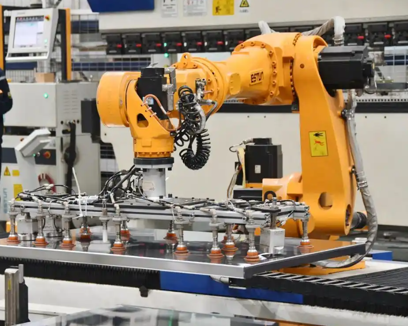
Digital twin-driven dynamic error modeling. I build the digital twin model to establish a precise virtual-real mirror mapping between the physical production line and the virtual model. The purpose is to synchronize equipment operation status and error parameters in a timely manner. My modeling process includes three closed-loop steps: virtual model construction, multi-type data collection, and real-time dynamic error fitting. During virtual model construction, I use the real structural dimensions of industrial robots, production-line layout, workstation coordinate datum, and planar operation path. I perform geometric modeling, kinematic modeling, and dynamic modeling in sequence. I strictly follow the real link lengths, joint limits, motion ranges, and installation relationships to achieve one-to-one high-precision restoration. This ensures that the virtual model accurately reflects the motion principle of industrial robots and the way errors are generated. It also provides a solid foundation for later error analysis and simulation calculation.
I represent the virtual model state as a vector:
$$ X_{dt}(t) = [q(t), \dot{q}(t), \ddot{q}(t), \tau(t), T(t), V(t), L(t), e(t)]^T $$
The physical state of industrial robots is represented by a corresponding vector:
$$ X_{phy}(t) = [q_m(t), \dot{q}_m(t), \ddot{q}_m(t), \tau_m(t), T_m(t), V_m(t), L_m(t), e_m(t)]^T $$
The synchronization error between the digital twin and the physical system is:
$$ e_{sync}(t) = X_{phy}(t) – X_{dt}(t) $$
I aim to minimize this synchronization error so that the virtual model can serve as a reliable observer for compensation. If \(e_{sync}(t)\) becomes large, the virtual model no longer reflects the real state of industrial robots, and the compensation command becomes unreliable.
I summarize the digital twin construction steps in the following table.
| Step | Input | Operation | Output |
|---|---|---|---|
| Virtual model construction | Structural dimensions, joint limits, layout, coordinate datum | Geometric, kinematic, and dynamic modeling of industrial robots | High-fidelity virtual robot and production line model |
| Multi-source data collection | Joint angles, pose, load, temperature, vibration | Sensor acquisition, bus transmission, filtering, time alignment | Clean time-series data set for error analysis |
| Real-time dynamic error fitting | Historical and current data | Hierarchical decoupling, machine learning, residual correction | Dynamic error model for industrial robots |
| Closed-loop update | Compensation result and new measurement | Parameter update, model refinement, synchronization check | Improved digital twin and compensation accuracy |
Multi-source error data acquisition. High-precision data acquisition is the foundation of accurate error modeling. I establish a multi-source heterogeneous data acquisition system. I use laser trackers, visual positioning modules, attitude sensors, temperature sensors, and vibration sensors. These devices comprehensively acquire joint angle information of industrial robots, end-effector position and attitude, real-time task load, environmental temperature variation, and vibration frequency of production equipment. All data from the production site are transmitted through an industrial bus to a twin data center for centralized processing, immediate archiving, and preliminary filtering. This allows real-time monitoring of the entire production line and provides a reliable basis for error separation, pattern summarization, and mathematical modeling.
I model the measurement process as:
$$ z_k = h(x_k) + v_k $$
where \(z_k\) is the measurement vector, \(x_k\) is the true state of industrial robots, \(h(\cdot)\) is the measurement function, and \(v_k\) is measurement noise. Because different sensors have different sampling rates, delays, and noise characteristics, I apply time alignment and data fusion. A general weighted least-squares fusion estimate is:
$$ \hat{x}_k = \arg\min_x \sum_{j=1}^{m} \| z_{k,j} – h_j(x) \|^2_{R_j} $$
where \(R_j\) is the measurement covariance of sensor \(j\). For real-time state estimation, I use a Kalman filter form:
$$ \hat{x}_{k|k} = \hat{x}_{k|k-1} + K_k (z_k – H_k \hat{x}_{k|k-1}) $$
$$ K_k = P_{k|k-1} H_k^T (H_k P_{k|k-1} H_k^T + R_k)^{-1} $$
This filtering framework helps suppress noise and improves the reliability of the digital twin for industrial robots. I also apply outlier rejection and missing-data imputation. Without these steps, sensor noise and packet loss can cause false error patterns and incorrect compensation.
The sensor types and their roles are summarized in the following table.
| Sensor type | Measured variable | Role in error modeling | Typical challenge |
|---|---|---|---|
| Laser tracker | End-effector position and pose | Provides high-accuracy ground truth for industrial robots | Line-of-sight blockage and setup cost |
| Visual positioning module | Pose and feature position | Supports online visual feedback and compensation verification | Lighting sensitivity and calibration drift |
| Attitude sensor | Orientation and angular velocity | Captures dynamic attitude deviation | Accumulated drift and magnetic interference |
| Temperature sensor | Joint, link, and ambient temperature | Models thermal deformation of industrial robots | Non-uniform temperature field |
| Vibration sensor | Vibration frequency and amplitude | Identifies environmental and structural disturbance | High-frequency noise and mounting effects |
| Joint encoder | Joint angle and velocity | Provides internal motion state of industrial robots | Resolution limits and quantization error |
| Load cell | Payload and torque | Captures load-induced deformation and dynamic error | Noise under impact and inertia |
Dynamic error fitting and hierarchical decoupling. To solve the problems of insufficient precision and weak generalization in traditional single modeling methods, I adopt a hierarchical decoupling approach to build a real-time iterative global dynamic error model. Traditional error modeling often relies only on pure kinematic algorithms to correct structural error. It ignores mechanical flexibility, temperature field coupling, load disturbance, and other cross-influences. Under complex industrial conditions, this easily leads to modeling distortion and compensation failure. My model completes error fitting in three layers. The first layer uses forward and inverse kinematics algorithms to correct fixed structural errors of industrial robots. The second layer introduces time-series machine learning algorithms to fit dynamic time-varying errors caused by temperature drift, load fluctuation, and equipment vibration. The third layer uses a residual correction algorithm to filter random interference errors at the production site.
I write the overall dynamic error model as:
$$ \hat{e}(t) = \hat{e}_{kin}(t) + \hat{e}_{dyn}(t) + \hat{e}_{res}(t) $$
The first-layer kinematic correction is:
$$ \hat{e}_{kin} = J(q) \Delta \xi $$
where \(J(q)\) is the Jacobian matrix of industrial robots and \(\Delta \xi\) is the identified kinematic parameter error. The second-layer dynamic prediction can be expressed as:
$$ \hat{e}_{dyn}(t) = f_{\theta}(e(t-1), e(t-2), \ldots, u(t), T(t), L(t), V(t)) $$
where \(f_{\theta}\) is a time-series model parameterized by \(\theta\), and \(u(t)\) is the control input. The third-layer residual correction is:
$$ \hat{e}_{res}(t) = g_{\phi}(r(t), s(t)) $$
where \(r(t)\) is the residual sequence and \(s(t)\) is the process context. The final compensated joint command is:
$$ q_{comp}(t) = q_{cmd}(t) – J^{-1}(q_{cmd}(t)) \hat{e}(t) $$
This equation is central to my compensation strategy. It shows that error prediction must be converted into joint-space correction through the inverse Jacobian. If the Jacobian is singular or ill-conditioned, I use a damped least-squares form:
$$ \Delta q = J^T (J J^T + \lambda^2 I)^{-1} \hat{e} $$
where \(\lambda\) is the damping factor. This improves numerical stability for industrial robots near singular configurations.
I summarize the hierarchical modeling layers in the following table.
| Layer | Error target | Method | Output | Adaptation speed |
|---|---|---|---|---|
| Layer 1 | Fixed structural error | Forward and inverse kinematics, parameter identification | Static kinematic correction | Slow, offline or periodic |
| Layer 2 | Dynamic time-varying error | Time-series machine learning, thermal and load features | Dynamic error prediction | Fast, online |
| Layer 3 | Random residual error | Residual correction, robust filtering | Random disturbance suppression | Real-time |
Intelligent compensation strategies based on the digital twin. I support the compensation design with digital twin virtual-real synchronization, simulation deduction, and data update iteration. I build a full-process closed-loop intelligent compensation mechanism: state perception, error prediction, precise compensation, and continuous optimization. The strategies of offline pre-compensation, online real-time compensation, and adaptive iterative compensation run through the entire life cycle of the production line, including debugging and installation, large-scale manufacturing, and later maintenance and repair.
Offline pre-compensation is mainly used in production-line debugging and equipment calibration. On the twin virtual platform, I simulate and calculate the basic positioning deviation under various motion trajectories and different load conditions. I then correct the kinematic parameters of industrial robots in advance and adjust the task path. This fundamentally eliminates fixed systematic deviation, significantly reduces the initial positioning deviation, and prepares the system for efficient and accurate processing.
I express offline pre-compensation as:
$$ q_{off} = q_{nom} + \Delta q_{kin} + \Delta q_{path} $$
where \(q_{nom}\) is the nominal joint command, \(\Delta q_{kin}\) is the kinematic parameter correction, and \(\Delta q_{path}\) is the path adjustment. The objective is to minimize the predicted error over a set of representative tasks:
$$ \min_{\Delta q_{kin}, \Delta q_{path}} \sum_{j=1}^{M} \| e_j(q_{off}) \|^2 $$
Online real-time compensation is the most important compensation method during batch production. It compensates for instantaneous dynamic deviation caused by working-condition changes. The twin system compares the real end-effector pose of the physical robot with the standard ideal pose of the virtual model in real time. It calculates the instantaneous positioning deviation immediately. According to the production-line working state, it adjusts the joint angle values and end-effector motion path of industrial robots in time. It eliminates instantaneous deviation caused by load mutation, equipment vibration, or external interference. This compensation method uses microsecond-level synchronization interaction between virtual and real systems. It integrates work, detection, and compensation into one process. It completely overcomes the problem of delayed post-event compensation and ensures that industrial robots maintain good positioning accuracy during continuous production.
I write online compensation as:
$$ q_{real}(t) = q_{cmd}(t) + \Delta q_{online}(t) $$
$$ \Delta q_{online}(t) = -J^{-1}(q_{cmd}(t)) \left( p_{real}(t) – p_{virtual}(t) \right) $$
where \(p_{real}(t)\) is the measured end-effector pose of industrial robots and \(p_{virtual}(t)\) is the ideal pose in the digital twin. The sign indicates that the correction is applied in the opposite direction of the detected error.
Adaptive iterative compensation mainly solves the error accumulation caused by slowly changing variables such as mechanical wear, structural aging, and temperature drift. These errors change slowly and are not easy to detect. In the short term, they do not have a large impact on precision. A single calibration can hardly remove them completely. However, as time goes on, they accumulate continuously. This causes the precision of industrial robots to decline and may lead to large-scale quality problems. Using the full-life-cycle data storage characteristics of the digital twin, the system continuously collects long-term error variation data. It forms a time-series database of equipment precision degradation. It uses incremental learning methods to update the parameters and compensation thresholds in the error model in real time. It automatically matches compensation schemes under different service cycles and work intensities.
I express adaptive iterative compensation as:
$$ \theta_{k+1} = \theta_k – \eta \nabla_{\theta} L(e_k, \hat{e}_k) $$
where \(\theta_k\) represents the adaptive model parameters, \(\eta\) is the learning rate, and \(L\) is the loss function. The compensation threshold is updated as:
$$ \delta_{k+1} = \delta_k + \alpha \left( \| e_k \| – \delta_k \right) $$
where \(\alpha\) is a smoothing factor. This allows industrial robots to gradually adapt to wear and aging without requiring a complete re-identification of the whole model.
I compare the three compensation strategies in the following table.
| Strategy | Application stage | Main target | Update frequency | Key advantage | Limitation |
|---|---|---|---|---|---|
| Offline pre-compensation | Debugging and calibration | Fixed systematic error | Low, offline | Eliminates initial bias and improves path accuracy | Cannot handle real-time disturbance |
| Online real-time compensation | Batch production | Instantaneous dynamic error | High, real-time | Suppresses load, vibration, and external disturbance | Depends on synchronization quality |
| Adaptive iterative compensation | Long-term operation and maintenance | Cumulative wear and aging error | Medium to low, iterative | Maintains accuracy over the life cycle | Requires long-term data and stable learning |
Engineering application effect verification. To verify the engineering practicality of my proposed scheme, I use the digital twin-based error modeling and intelligent compensation method in an industrial robot precision assembly production line for experimental validation. The experimental results show that compared with traditional manual fixed calibration compensation, my technology can improve the end-effector positioning accuracy of industrial robots by more than sixty percent. It greatly improves the consistency of repositioning. It effectively solves the problems of misalignment, poor fitting, and dimensional exceedance in precision assembly. It significantly improves the product qualification rate. The technology also enables real-time online self-calibration without stopping the equipment. It avoids the production time loss required by traditional periodic calibration. To a certain extent, it reduces production-line downtime loss and manual maintenance cost. It significantly improves the overall operation efficiency and intelligent maintenance level of the automated production line.
I quantify the improvement with the following equations. If the original positioning error is \(E_{before}\) and the compensated error is \(E_{after}\), the accuracy improvement is:
$$ \eta_{acc} = \left( 1 – \frac{E_{after}}{E_{before}} \right) \times 100\% $$
The repeatability improvement is:
$$ \eta_{rep} = \left( 1 – \frac{\sigma_{after}}{\sigma_{before}} \right) \times 100\% $$
where \(\sigma\) is the standard deviation of repeated positioning. The downtime reduction is:
$$ \eta_{down} = \frac{T_{cal, before} – T_{cal, after}}{T_{cal, before}} \times 100\% $$
where \(T_{cal}\) is the calibration downtime. These metrics provide a clear view of both technical and economic benefits for industrial robots.
I summarize a representative validation result in the following table. The values are expressed as relative indicators because they depend on the specific production line and task.
| Metric | Traditional fixed calibration | Digital twin intelligent compensation | Relative improvement |
|---|---|---|---|
| End-effector positioning error | Baseline | Reduced significantly | More than 60% reduction |
| Repositioning consistency | Moderate | High | Substantial improvement |
| Assembly misalignment rate | Higher | Lower | Clear quality improvement |
| Product qualification rate | Baseline | Improved | Significant increase |
| Calibration downtime | Periodic stoppage required | Online self-calibration | Reduced downtime |
| Manual maintenance cost | Higher | Lower | Cost reduction |
| Operation and maintenance intelligence | Reactive | Predictive and adaptive | Improved autonomy |
Core technical advantages. Compared with traditional error correction methods, my digital twin-based intelligent compensation system has obvious technical advantages. First, error control is comprehensive. It can simultaneously address static systematic error, dynamic deformation error, and random working-condition error. It solves the previous problem that only a single static error could be corrected. Second, error compensation is immediate. On the basis of virtual-real synchronization, it completes error discovery, calculation, and real-time compensation instantly. It effectively avoids delayed compensation. It is suitable for high-speed, continuous, and high-precision production lines of industrial robots. Third, the management mode is automatic. Under equipment aging or environmental change, it automatically optimizes the corresponding model parameters and compensation scheme. It reduces the influence of human operation.
I further formalize the comprehensive error control objective as a multi-objective optimization problem:
$$ \min_{q} \left( w_1 \| e_{kin} \|^2 + w_2 \| e_{dyn} \|^2 + w_3 \| e_{env} \|^2 + w_4 \| \Delta q \|^2 \right) $$
where \(w_1, w_2, w_3, w_4\) are weights, and \(\Delta q\) is the compensation effort. The last term is important because excessive compensation can cause joint jerk, oscillation, or unnecessary wear in industrial robots. Therefore, I balance accuracy improvement with motion smoothness and actuator load.
I summarize the comparison between traditional methods and my digital twin method in the following table.
| Aspect | Traditional fixed calibration | Digital twin intelligent compensation |
|---|---|---|
| Error types addressed | Mainly static systematic error | Static, dynamic, and random error |
| Response speed | Slow, periodic | Real-time, microsecond-level synchronization |
| Adaptability | Weak | Strong, model updates automatically |
| Human intervention | High | Low |
| Production interruption | Required for calibration | Online self-calibration without stopping |
| Long-term accuracy | Degrades with wear and aging | Maintained by adaptive iterative compensation |
| Suitability for industrial robots | Limited to stable ideal conditions | Designed for complex industrial conditions |
Current difficulties in technical application. At present, digital twin error modeling and intelligent compensation technology still has many bottlenecks in industrial implementation. First, virtual-real synchronization accuracy is insufficient. Sensors in industrial sites are prone to signal noise, data transmission delay, and packet loss. This causes time-sequence inconsistency between the virtual model and physical equipment. It becomes difficult to accurately identify subtle positioning deviation. This affects the accuracy of error modeling for industrial robots. Second, multi-robot error separation is difficult. In a multi-robot coordinated production line, each equipment node restricts the others, and errors are intertwined. It is impossible to effectively distinguish single-machine equipment error from workstation coordination error. This greatly limits the overall error compensation effect. Third, the cost of technology implementation is relatively high. The construction and later maintenance of high-precision perception equipment and twin simulation systems require large investment. The technical application threshold is high, and it is difficult to popularize among small and medium-sized manufacturing enterprises.
I also note that model complexity can become a barrier. A very detailed digital twin may require significant computing resources. If the model is too complex, the online compensation loop may not meet real-time requirements. Therefore, there is a trade-off between model fidelity and computational latency. I express this trade-off as:
$$ \min_{M} \left( \alpha \| e(M) \|^2 + \beta C(M) + \gamma \tau(M) \right) $$
where \(M\) is the model structure, \(C(M)\) is computational cost, \(\tau(M)\) is latency, and \(\alpha, \beta, \gamma\) are weights. This equation captures the practical need for lightweight digital twins that still provide accurate compensation for industrial robots.
I summarize the main difficulties and their effects in the following table.
| Difficulty | Root cause | Effect on industrial robots | Potential countermeasure |
|---|---|---|---|
| Insufficient virtual-real synchronization | Sensor noise, transmission delay, packet loss | Inaccurate subtle error identification | Filtering, outlier removal, time alignment |
| Multi-robot error separation | Coupling between robots and workstations | Single-machine error cannot be distinguished from coordination error | Block modeling, correlation analysis, traceability |
| High implementation cost | Expensive sensors, simulation systems, maintenance | Limited adoption in small and medium enterprises | Simplified twin architecture and standard sensors |
| Model complexity | High-fidelity simulation requires computation | Real-time compensation latency may increase | Reduced-order modeling and edge computing |
| Long-term data stability | Changing production tasks and environments | Adaptive model may drift | Incremental learning with validation gates |
Targeted optimization measures. In response to the above problems, I propose several engineering optimization solutions to improve the technical application effect. First, I optimize the data preprocessing system. I use filtering and denoising, abnormal data elimination, data imputation, and time-sequence synchronization to standardize the processing of field data. This improves data quality and virtual-real time-sequence consistency. It strengthens the ability to detect and model small errors. Second, I build a multi-robot error separation mechanism. Relying on block modeling, correlation analysis, and backtracking methods, I distinguish single-machine error from multi-station coordinated comprehensive error. I clarify the cause of error and its influence weight. This realizes comprehensive correction of the overall production-line error. Third, I simplify the twin model architecture. I remove redundant simulation parameters and adapt to conventional factory sensor equipment. This reduces construction and operation and maintenance costs. I also combine artificial intelligence early-warning technology to realize error prediction and intelligent regulation. This improves the autonomous error-correction ability of the system and helps the technology achieve large-scale application.
I further propose a staged deployment strategy. In the first stage, I use offline pre-compensation to correct fixed kinematic errors of industrial robots. In the second stage, I add online real-time compensation for dynamic disturbance. In the third stage, I enable adaptive iterative compensation for long-term wear and aging. This staged approach reduces initial investment and allows the system to grow with the production line. I express the staged performance improvement as:
$$ E_{stage}(t) = E_0 \prod_{s=1}^{S} \left( 1 – \rho_s(t) \right) $$
where \(E_0\) is the initial error, \(S\) is the number of deployed stages, and \(\rho_s(t)\) is the error reduction ratio of stage \(s\). This model helps me plan the expected accuracy improvement without overbuilding the digital twin at the beginning.
I also recommend a validation gate for adaptive updates. Before a new model parameter is deployed to industrial robots, it must pass a validation set:
$$ \| e_{val}( \theta_{new} ) \| < \| e_{val}( \theta_{old} ) \| + \kappa $$
where \(\kappa\) is a tolerance margin. If the condition is not met, the update is rejected. This prevents negative transfer and protects production stability.
I summarize the optimization measures and expected outcomes in the following table.
| Optimization measure | Implementation method | Expected outcome for industrial robots |
|---|---|---|
| Data preprocessing optimization | Filtering, outlier removal, imputation, time alignment | Higher data quality and more reliable error modeling |
| Multi-robot error separation | Block modeling, correlation analysis, backtracking | Clear separation of single-machine and coordination error |
| Lightweight twin architecture | Remove redundant parameters, use standard sensors | Lower cost and easier deployment |
| Artificial intelligence early warning | Error prediction and intelligent regulation | Improved autonomous error correction |
| Staged deployment | Offline, online, then adaptive compensation | Controlled investment and scalable accuracy improvement |
| Validation gate | Compare new and old models on validation data | Stable adaptation without negative transfer |
Conclusion. Digital twin technology uses virtual-real synchronous mapping, dynamic information collection, and simulation-computing update characteristics to overcome the limitations of previous precision management methods. It can perform dynamic modeling, instant correction, and automatic adjustment and update of the positioning deviation of industrial robots. It solves coupled errors caused by multiple factors, lagging error management caused by time variation, and performance degradation of equipment during long-term use. It greatly improves the working accuracy of industrial robots and the stability of the production line. In my analysis, the key to success is not a single algorithm but the integration of error source classification, multi-source data acquisition, hierarchical dynamic fitting, and staged intelligent compensation. When these elements are combined, industrial robots can maintain high positioning accuracy under complex production conditions. The digital twin becomes not only a simulation tool but also a real-time accuracy-control infrastructure for modern intelligent manufacturing.
From my perspective, the future development of this technology should focus on three directions. The first direction is robust synchronization under imperfect industrial networks. The second direction is scalable multi-robot error separation with interpretable models. The third direction is low-cost and lightweight digital twin deployment for small and medium-sized enterprises. If these directions are addressed, the positioning accuracy of industrial robots can be managed as a continuously optimized life-cycle property rather than a periodically recalibrated static parameter. This is the most promising path I see for digital twin-driven error modeling and intelligent compensation in industrial robot production lines.