
In this review I examine the state of the art in motion reliability for industrial robots, with the aim of unifying the vocabulary, the mathematical models, and the computational strategies that have appeared across the literature. Industrial robots are now core assets in intelligent manufacturing, and their ability to repeat a task with high accuracy while tolerating manufacturing tolerances, assembly errors, wear, and joint clearances determines whether a production line can meet its quality targets. I structure the discussion around two complementary notions: point reliability, which quantifies the probability that the end effector remains inside a permissible error region at a specific instant, and time-varying reliability, which quantifies the probability that the entire trajectory remains inside that region throughout a task interval. I then build the kinematic and error models that support both notions, analyze the main solution techniques, and outline the directions that I believe will dominate future work on industrial robots.
Why Motion Reliability Matters for Industrial Robots
The deployment of industrial robots in welding, drilling, engraving, assembly, painting, and medical procedures has created a demand for quantitative statements about how well a robot performs under uncertainty. A robot that is nominally precise may still fail to satisfy a tolerance requirement when link dimensions deviate from their nominal values, when gear transmission introduces backlash, or when thermal effects alter the geometry of the arm. Because these perturbations accumulate along the kinematic chain, the pose of the end effector drifts away from the commanded pose, and the drift may exceed the tolerance band that the process can accept. Motion reliability provides the probabilistic language needed to describe this situation and to compare design alternatives for industrial robots on a common footing.
I treat reliability as a performance attribute rather than a purely mechanical property. In my view, the motion reliability of industrial robots is a system-level characteristic that couples mechanical design, control architecture, sensing, and operating conditions. This coupling is why a single deterministic error bound is rarely sufficient: the same robot may be perfectly reliable for a spot-welding operation and unreliable for a high-precision drilling operation, even though both tasks are executed by the same machine. The difference lies in the tolerance band, the trajectory, and the duration of the task.
| Source of uncertainty | Physical origin | Typical effect on the end effector | Time dependence |
|---|---|---|---|
| Link dimension deviation | Manufacturing tolerances | Static offset in position | Slow drift, usually constant |
| Joint clearance | Assembly clearances, wear | Backlash and non-smooth error | Grows with operating time |
| Gear transmission error | Tooth profile deviation, backlash | Periodic angular error | Periodic, load dependent |
| Elastic deformation | Payload and inertial loads | Configuration-dependent deflection | Varies within a motion cycle |
| Thermal expansion | Motor heating, ambient temperature | Slow geometric drift | Slow, cumulative |
| Control and sensing error | Encoder resolution, servo lag | Tracking error along the path | Continuous during motion |
The table above summarizes the dominant uncertainty sources that I consider when constructing a reliability model for industrial robots. Geometric errors usually dominate in stable workshop environments, while wear and thermal effects become important for long duty cycles. I therefore recommend that any reliability assessment of industrial robots begin with an explicit inventory of uncertainty sources, because the choice of model structure and the choice of solution algorithm both depend on which sources are retained.
Fundamental Definitions and Metrics
I define motion reliability as the probability that the end effector of an industrial robot satisfies a specified accuracy requirement over a specified domain. The domain may be a single instant, in which case I speak of point reliability, or it may be a time interval, in which case I speak of time-varying reliability. This distinction is not merely terminological. Point reliability is appropriate when the task consists of discrete positioning operations, such as rapid pick-and-place or spot welding, where the robot must be accurate at a finite set of configurations. Time-varying reliability is appropriate when the task consists of continuous path operations, such as arc welding, spraying, polishing, or surgical assistance, where the accuracy must be maintained along the entire trajectory.
Let the commanded pose of the end effector be denoted by a six-dimensional vector, and let the actual pose be denoted by another six-dimensional vector. The pose error is the difference between them, and I write it as
$$ \Delta \mathbf{p} = \mathbf{p}_a – \mathbf{p}_d = \left[ \Delta x, \Delta y, \Delta z, \Delta \alpha, \Delta \beta, \Delta \gamma \right]^{T} $$
The magnitude of this error can be aggregated into a scalar measure. A common choice is the squared norm that combines the three position components and the three orientation components,
$$ \delta^2 = \Delta x^2 + \Delta y^2 + \Delta z^2 + \Delta \alpha^2 + \Delta \beta^2 + \Delta \gamma^2 $$
With this scalar measure, point reliability is the probability that the squared error remains below the squared tolerance radius,
$$ R = \Pr\left\{ \delta^2 < r^2 \right\} $$
and the corresponding failure probability is the complementary event,
$$ p_f = \Pr\left\{ \delta^2 \ge r^2 \right\} = 1 – R $$
When the error components are approximately normal and independent, the normalized squared error follows a chi-square distribution, and the point reliability can be written in closed form as
$$ R = \Pr\left\{ \chi_{6}^{2} < \frac{r^2}{\sigma^2} \right\} $$
where \( \sigma \) denotes the common standard deviation of the normalized components and \( \chi_{6}^{2} \) is the chi-square variable with six degrees of freedom. This expression is convenient for preliminary design studies of industrial robots, because it allows the designer to trade tolerance radius against error variance without repeated simulation.
| Aspect | Point reliability | Time-varying reliability |
|---|---|---|
| Domain | A single instant or a finite set of instants | A continuous time interval |
| Mathematical form | Probability of a static event | Probability of an intersection of events |
| Typical index | \( \delta^2 < r^2 \) | \( \bigcap_{j} |g_j| \le \varepsilon \) for all \( t \) |
| Representative tasks | Spot welding, drilling, rapid positioning | Arc welding, spraying, polishing, surgery |
| Main limitation | Ignores failure at other points on the path | Requires more complex algorithms |
| Engineering value | Fast screening and comparison | Realistic assessment of continuous operations |
Kinematic Modeling of Industrial Robots
Any reliability assessment of industrial robots must rest on a kinematic model that maps joint variables to end-effector pose. I adopt the Denavit-Hartenberg convention as the baseline because it provides a systematic procedure for attaching a coordinate frame to each link and for expressing the transformation between adjacent frames with four parameters: link length, link twist, link offset, and joint angle. For a serial manipulator with \( n \) joints, the transformation from frame \( i-1 \) to frame \( i \) is
$$ T_{i}^{i-1} = \begin{bmatrix} \cos\theta_i & -\sin\theta_i\cos\alpha_i & \sin\theta_i\sin\alpha_i & a_i\cos\theta_i \\ \sin\theta_i & \cos\theta_i\cos\alpha_i & -\cos\theta_i\sin\alpha_i & a_i\sin\theta_i \\ 0 & \sin\alpha_i & \cos\alpha_i & d_i \\ 0 & 0 & 0 & 1 \end{bmatrix} $$
The forward kinematics of the complete chain is obtained by multiplying the individual transformations,
$$ T_{n}^{0}(\mathbf{q}) = \prod_{i=1}^{n} T_{i}^{i-1}(q_i) $$
and the pose of the end effector is extracted from the resulting homogeneous matrix,
$$ \mathbf{p}_e = \mathbf{f}(\mathbf{q}) = \left[ x(\mathbf{q}), y(\mathbf{q}), z(\mathbf{q}), \alpha(\mathbf{q}), \beta(\mathbf{q}), \gamma(\mathbf{q}) \right]^{T} $$
The classical convention places the frame of joint \( i \) at the distal end of link \( i \). A modified convention places it at the proximal end, which makes the correspondence between frames and joints more intuitive and reduces the likelihood of modeling mistakes when the number of joints grows. I use the modified convention whenever the kinematic structure is complex, and I note that the choice of convention does not change the physical reliability results as long as the error model is derived consistently.
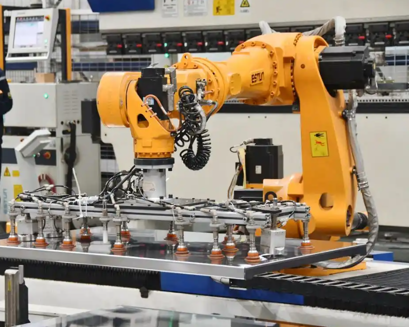
The kinematic model is the foundation on which every subsequent reliability calculation is built. If the kinematic model is inconsistent with the physical geometry of the industrial robot, then the error model will inherit that inconsistency, and the resulting reliability estimate will be biased regardless of how sophisticated the solution algorithm becomes. For this reason I recommend that the kinematic model be validated against a calibration experiment before it is used for reliability prediction.
| Feature | Standard convention | Modified convention |
|---|---|---|
| Frame attachment | Distal end of the link | Proximal end of the link |
| Interpretation | Convenient for matrix algebra | More intuitive for joint reasoning |
| Parameter count | Four per joint | Four per joint |
| Modeling risk | Higher for long chains | Lower for long chains |
| Use in reliability work | Widely used as a baseline | Preferred when clarity matters |
Error Modeling and Uncertainty Propagation
Given a kinematic model, the next step in the reliability analysis of industrial robots is to describe how parametric errors propagate to the end effector. I express the pose error as a truncated Taylor expansion of the forward kinematic function around the nominal joint vector,
$$ \Delta \mathbf{p} = \mathbf{J}(\mathbf{q}) \Delta \mathbf{q} + \frac{1}{2} \sum_{i=1}^{n} \sum_{j=1}^{n} \frac{\partial^2 \mathbf{f}}{\partial q_i \partial q_j} \Delta q_i \Delta q_j + \cdots $$
where the Jacobian matrix is
$$ \mathbf{J}(\mathbf{q}) = \frac{\partial \mathbf{f}(\mathbf{q})}{\partial \mathbf{q}} \in \mathbb{R}^{6 \times n} $$
The linear term dominates when the perturbations are small, which is usually the case for industrial robots operating in controlled environments. The quadratic term becomes relevant when joint clearances are large or when the manipulator operates near a singular configuration. I therefore retain the quadratic term in the error model whenever the clearance-to-link-length ratio exceeds a threshold that I set according to the required accuracy level.
Parameter errors enter the model through the four Denavit-Hartenberg parameters of each joint. If the vector of geometric parameters is denoted by \( \boldsymbol{\xi} \), the pose error can be expressed as
$$ \Delta \mathbf{p} = \mathbf{J}_{\xi}(\mathbf{q}, \boldsymbol{\xi}) \Delta \boldsymbol{\xi} + \mathbf{J}(\mathbf{q}) \Delta \mathbf{q} $$
where \( \mathbf{J}_{\xi} \) is the sensitivity matrix of the pose with respect to the geometric parameters. This decomposition is useful because it separates geometric errors, which are constant for a given unit, from joint-space errors, which vary during operation. For industrial robots that are calibrated periodically, the geometric component shrinks after each calibration, while the joint-space component persists.
| Error component | Mathematical representation | Dominant in |
|---|---|---|
| Geometric parameter error | \( \mathbf{J}_{\xi} \Delta \boldsymbol{\xi} \) | Uncalibrated or newly assembled robots |
| Joint clearance error | Nonlinear function of clearance vector | Worn joints, high-load operations |
| Elastic deformation | Stiffness-dependent deflection | Heavy payloads, long reaches |
| Thermal drift | Time-varying offset vector | Long duty cycles |
| Servo tracking error | Frequency-dependent transfer function | High-speed trajectories |
In my experience, the most delicate part of error modeling for industrial robots is the treatment of joint clearances. A clearance introduces a discontinuity in the effective joint variable, and this discontinuity interacts with the direction of motion. As a result, the error contribution of a clearance is not a simple additive term but a state-dependent quantity that must be evaluated along the trajectory. Some authors handle this by augmenting the kinematic chain with additional virtual joints, which converts the clearance into a continuous parameter at the cost of increasing the dimension of the model. I find this approach attractive because it preserves the smoothness of the reliability formulation.
Point Reliability Formulation
Point reliability for industrial robots is formulated by treating the tolerance requirement as a spherical acceptance region in the six-dimensional error space. The acceptance region is centered on the commanded pose, and its radius is the permissible error magnitude. The event of interest is that the actual pose falls inside this region. The reliability is the probability of that event, and the failure probability is the probability of the complement.
The standard assumption in the literature is that the error components are jointly normal with zero mean and a covariance matrix that can be estimated from manufacturing data. Under this assumption, the squared error \( \delta^2 \) is a quadratic form in normal variables, and its distribution can be characterized either exactly or through a chi-square approximation. The exact characterization uses the eigenvalues of the covariance matrix, while the chi-square approximation assumes equal variances across components. I prefer the eigenvalue-based approach when the covariance matrix is available, because it captures anisotropy in the error distribution.
$$ \delta^2 = \sum_{k=1}^{6} \lambda_k \chi_{1,k}^{2} $$
In this expression, \( \lambda_k \) are the eigenvalues of the covariance matrix and \( \chi_{1,k}^{2} \) are independent chi-square variables with one degree of freedom. The reliability is then obtained by integrating the corresponding distribution up to the tolerance radius.
Point reliability is particularly convenient for tasks such as drilling, where the robot must position a tool at a sequence of discrete locations with a specified positional tolerance. I can compute the reliability at each location and then combine the results under an independence assumption, or I can treat the locations as a series system and compute the probability that all of them succeed. The series-system formulation is conservative but simple, and it provides a useful upper bound on the true reliability of the task.
$$ R_{\text{task}} = \prod_{k=1}^{m} R_k $$
The product form is valid only when the errors at different locations are statistically independent, which is not always true for industrial robots because geometric errors are shared across configurations. A more accurate approach is to treat the geometric parameters as common random variables and the configuration-specific errors as conditionally independent. I recommend this hierarchical structure because it reflects the physical reality of industrial robots better than a purely independent model.
Time-Varying Reliability Formulation
Time-varying reliability extends the point formulation to the entire task interval. The event of interest is that the end effector remains inside the tolerance region at every instant between the start time and the end time. This is an intersection of uncountably many events, and it is the reason why time-varying reliability is mathematically more demanding than point reliability.
$$ R(t_0, t_e) = \Pr\left\{ \bigcap_{j=1}^{6} \left| g_j(\mathbf{X}, \theta, t) \right| \le \varepsilon, \ \forall t \in [t_0, t_e] \right\} $$
A convenient way to rewrite this expression is to introduce a limit-state function that is positive when the requirement is satisfied and negative when it is violated,
$$ Z(t) = \varepsilon – \left\| \mathbf{p}_a(t) – \mathbf{p}_d(t) \right\| $$
The trajectory is reliable if and only if the minimum of \( Z(t) \) over the interval is positive. This observation converts the time-varying problem into an extreme-value problem,
$$ R(t_0, t_e) = \Pr\left\{ \min_{t \in [t_0, t_e]} Z(t) > 0 \right\} $$
The extreme-value formulation is the conceptual bridge between time-varying reliability and the envelope method. If I can construct an envelope that bounds the error over the interval, then the minimum of the limit-state function over the interval is bounded by the minimum of the envelope, and the reliability calculation becomes a static calculation on the envelope.
The first-passage formulation takes a different route. It models the limit-state function as a random process and computes the rate at which the process crosses the zero level from the safe side to the unsafe side. The failure probability over the interval is then approximated by an exponential function of the integrated crossing rate,
$$ p_f(t_0, t_e) \approx 1 – \exp\left( -\int_{t_0}^{t_e} \nu^{+}(t) \, dt \right) $$
where the crossing rate is given by the Rice formula,
$$ \nu^{+}(t) = \int_{0}^{\infty} \dot{z} \, f_{Z\dot{Z}}(0, \dot{z}, t) \, d\dot{z} $$
The Rice formula requires the joint density of the process and its derivative at the zero level. For Gaussian processes this density is available in closed form, which is why the first-passage method is attractive for industrial robots whose error processes are approximately Gaussian. When the process is non-Gaussian, the joint density must be estimated, and the accuracy of the method depends on the quality of that estimate.
Solution Methods for Motion Reliability
I now turn to the computational methods that are used to evaluate the reliability models described above. I group them into four families: Monte Carlo simulation, the envelope method, the first-order second-moment method, and the first-passage method. Each family has a distinct position in the trade-off between accuracy and cost, and I summarize the trade-off in the table below before discussing each family in detail.
| Method | Core idea | Computational cost | Accuracy | Best suited for |
|---|---|---|---|---|
| Monte Carlo simulation | Random sampling and statistical estimation | High | Very high | Benchmarking and validation |
| Envelope method | Conversion of a dynamic problem into a static geometric bound | Moderate | Moderate, often conservative | Continuous trajectories |
| First-order second-moment method | Linearization at a design point | Low | Moderate, sensitive to nonlinearity | Rapid screening of industrial robots |
| First-passage method | Integration of the threshold crossing rate | Moderate | Depends on process assumptions | Time-varying reliability of continuous paths |
Monte Carlo Simulation
Monte Carlo simulation is the most direct method for assessing the motion reliability of industrial robots. I generate a large number of random realizations of the uncertain parameters, evaluate the forward kinematics for each realization, and count the fraction of realizations that satisfy the tolerance requirement. The estimator is
$$ \hat{R} = \frac{1}{N} \sum_{i=1}^{N} \mathbf{1}\left[ \delta^2(\mathbf{X}_i) < r^2 \right] $$
The statistical properties of this estimator are well understood. It is unbiased, and its variance is
$$ \mathrm{Var}\left( \hat{R} \right) = \frac{R(1-R)}{N} $$
The coefficient of variation is therefore
$$ \mathrm{COV} = \frac{\sqrt{\mathrm{Var}(\hat{R})}}{R} = \sqrt{\frac{1-R}{N R}} $$
This expression shows that the number of samples required to achieve a given relative accuracy grows rapidly as the reliability approaches one. For a reliability of 0.999 and a target coefficient of variation of 0.05, the required number of samples is on the order of four hundred thousand. For industrial robots with very high reliability requirements, this cost can be prohibitive, which is why variance reduction techniques such as importance sampling and subset simulation are often employed.
| Reliability \( R \) | Target COV | Approximate samples required |
|---|---|---|
| 0.900 | 0.05 | 4.4 × 10² |
| 0.990 | 0.05 | 4.0 × 10³ |
| 0.999 | 0.05 | 4.0 × 10⁴ |
| 0.9999 | 0.05 | 4.0 × 10⁵ |
Despite its cost, Monte Carlo simulation remains the reference against which I validate other methods. When a new analytical or semi-analytical technique is proposed for industrial robots, the first question I ask is whether it agrees with a well-designed Monte Carlo study over a range of operating conditions. Agreement in a single scenario is not sufficient, because the accuracy of approximate methods depends on the nonlinearity of the limit-state function, and that nonlinearity varies across the workspace.
Envelope Method
The envelope method is the technique that I find most natural for continuous-path operations. The idea is to replace the time-dependent error by a time-independent envelope that bounds the error over the interval, so that the dynamic reliability problem becomes a static reliability problem. If the envelope is denoted by \( E(\mathbf{X}) \), the reliability is
$$ R = \Pr\left\{ E(\mathbf{X}) < r \right\} $$
The construction of the envelope is the critical step. A conservative envelope is easy to build but produces an underestimate of reliability, while a tight envelope requires more computation but produces a more accurate result. In practice I use a combination of interval arithmetic and sensitivity analysis to build an envelope that is both tight and inexpensive to evaluate.
$$ E(\mathbf{X}) = \max_{t \in [t_0, t_e]} \left\| \mathbf{p}_a(\mathbf{X}, t) – \mathbf{p}_d(t) \right\| $$
The envelope method is particularly effective for industrial robots that execute repetitive trajectories, because the envelope can be computed once for a given trajectory and then reused for many reliability evaluations with different parameter distributions. This reuse is a significant computational advantage in design optimization, where the same trajectory is evaluated thousands of times.
First-Order Second-Moment Method
The first-order second-moment method is the workhorse of engineering reliability analysis, and it is widely applied to industrial robots because of its simplicity. The method linearizes the limit-state function at a design point and uses the first two moments of the random variables to compute a reliability index. The linearization is
$$ g(\mathbf{X}) \approx g(\mathbf{X}^{*}) + \nabla g(\mathbf{X}^{*})^{T} \left( \mathbf{X} – \mathbf{X}^{*} \right) $$
where \( \mathbf{X}^{*} \) is the design point, usually taken as the most probable failure point. The mean and standard deviation of the linearized function are
$$ \mu_g \approx g(\boldsymbol{\mu}_X) $$
$$ \sigma_g^2 \approx \sum_{i=1}^{n} \left( \frac{\partial g}{\partial X_i} \bigg|_{\boldsymbol{\mu}_X} \right)^{2} \sigma_{X_i}^{2} $$
The reliability index is the ratio of the mean to the standard deviation,
$$ \beta = \frac{\mu_g}{\sigma_g} $$
and the failure probability is approximated by the standard normal cumulative distribution,
$$ p_f \approx \Phi(-\beta), \qquad R \approx \Phi(\beta) $$
The method is fast and requires only first-order derivative information, which can be obtained analytically from the Jacobian of the kinematic model. Its weakness is that it ignores the curvature of the limit-state function. For industrial robots operating near singular configurations, where the curvature is large, the first-order second-moment method can produce significant errors. I therefore use it as a screening tool and reserve more accurate methods for configurations that the screening identifies as critical.
First-Passage Method
The first-passage method is the most natural formulation for the time-varying reliability of industrial robots, because it directly addresses the question of when the error process first exceeds the tolerance threshold. The method requires the crossing rate, which for a Gaussian process can be computed analytically,
$$ \nu^{+}(t) = \frac{\sigma_{\dot{Z}}(t)}{2\pi \sigma_{Z}(t)} \exp\left( -\frac{\mu_{Z}^{2}(t)}{2\sigma_{Z}^{2}(t)} \right) $$
where \( \mu_Z \), \( \sigma_Z \), and \( \sigma_{\dot{Z}} \) are the mean, standard deviation, and derivative standard deviation of the limit-state process. The failure probability over the interval is then
$$ p_f(t_0, t_e) \approx 1 – \exp\left( -\int_{t_0}^{t_e} \nu^{+}(t) \, dt \right) $$
The accuracy of this approximation depends on the assumption that crossings are rare and independent, which is reasonable for high-reliability industrial robots but questionable when the error process exhibits clustering or when the tolerance threshold is close to the mean error. In those cases I recommend a simulation-based correction or a more refined process model.
Advanced Uncertainty Representations
The methods described so far assume that the uncertain parameters are described by probability distributions. In practice, some parameters of industrial robots are known only within intervals, either because the available data are insufficient to fit a distribution or because the parameter is specified as a tolerance range. Ignoring this distinction and forcing a probability distribution onto an interval parameter can produce misleading reliability estimates. I therefore consider three alternative representations: interval variables, evidence variables, and fuzzy variables, and I summarize their roles in the table below.
| Representation | Information required | Output form | Typical use for industrial robots |
|---|---|---|---|
| Probabilistic | Full distribution | Single probability | Manufactured batches with quality data |
| Interval | Bounds only | Interval of reliability | Early design with limited data |
| Evidence | Basic probability assignment | Belief and plausibility bounds | Mixed aleatory and epistemic uncertainty |
| Fuzzy | Membership function | Fuzzy reliability | Expert judgment on wear and environment |
When aleatory and epistemic uncertainties coexist, I find that a combined probability-evidence formulation is the most informative. The random variables are treated probabilistically, the evidence variables are treated by means of basic probability assignments, and the final result is reported as an interval of reliability rather than a single number. This interval communicates the limits of what can be inferred from the available data, which is important when the reliability assessment supports a safety-related decision about industrial robots.
$$ R \in \left[ R_{\text{bel}}, R_{\text{pl}} \right] $$
The belief and plausibility bounds bracket the true reliability, and their width is a measure of the epistemic uncertainty. Narrow bounds indicate that the available data are sufficient to support a confident reliability statement, while wide bounds indicate that additional testing or calibration is needed before a decision can be made.
Sensitivity Analysis and Parameter Importance
A reliability estimate is only useful if it can be traced back to the parameters that drive it. Sensitivity analysis provides that trace. I define the sensitivity of reliability with respect to a parameter as the partial derivative of the reliability index with respect to that parameter, normalized by the parameter value,
$$ S_{i} = \frac{\partial \beta}{\partial \theta_{i}} \frac{\theta_{i}}{\beta} $$
This normalized measure allows me to compare parameters with different physical units and to rank them by their influence on the reliability of industrial robots. In my experience, the ranking is often counterintuitive. Link lengths may dominate the positional error, while joint clearances may dominate the orientational error, and the relative importance of the two depends on the configuration and on the tolerance radius.
| Parameter | Effect on position error | Effect on orientation error | Practical controllability |
|---|---|---|---|
| Link length | High, accumulates along the chain | Low to moderate | Fixed at manufacture, adjustable by calibration |
| Link twist | Moderate | High | Fixed at manufacture |
| Joint offset | Moderate | Moderate | Calibration can partially correct |
| Joint angle error | High, configuration dependent | High, configuration dependent | Controllable through servo tuning |
| Joint clearance | Moderate to high | Moderate to high | Reduced by preload and maintenance |
The sensitivity results also inform the design of experiments. If a small number of parameters dominate the reliability of industrial robots, then the calibration effort should focus on those parameters, and the testing budget should be allocated accordingly. This is a more efficient use of resources than a uniform calibration effort, which spreads the budget thinly across parameters that may have little influence.
Applications and Requirements in Manufacturing
The reliability requirements of industrial robots depend strongly on the application. I summarize the typical requirements and the corresponding reliability formulations in the table below. The requirements are expressed in terms of the tolerance radius and the task duration, and the formulation column indicates whether point reliability or time-varying reliability is the appropriate framework.
| Application | Dominant error concern | Task character | Preferred reliability formulation |
|---|---|---|---|
| Spot welding | Position at discrete points | Discrete | Point reliability |
| Drilling | Position and orientation at entry | Discrete with short moves | Point reliability |
| Arc welding | Continuous path accuracy | Continuous | Time-varying reliability |
| Spraying | Path and velocity consistency | Continuous | Time-varying reliability |
| Polishing | Contact force and path accuracy | Continuous with load variation | Time-varying reliability |
| Assembly | Fine positioning and orientation | Discrete with compliance | Point reliability with contact model |
| Engraving | Path fidelity and depth control | Continuous | Time-varying reliability |
For arc welding and spraying, the time-varying formulation is essential because the quality of the deposit depends on the accuracy of the entire path, not just on the accuracy at the endpoints. For assembly, the point formulation is usually sufficient, but the tolerance radius must account for the compliance of the parts and for the clearance in the mating interface. I find that the most common mistake in industrial practice is to apply a point-reliability criterion to a continuous-path task, which produces an optimistic estimate because it ignores the possibility of failure between the sampled points.
Machine Learning and Surrogate Modeling
The computational cost of reliability analysis for industrial robots grows rapidly with the number of uncertain parameters and with the number of trajectory points. Surrogate modeling addresses this cost by replacing the expensive forward kinematic model with a cheap approximation that is trained on a limited number of exact evaluations. I use Kriging surrogates in my own work because they provide both a prediction and an uncertainty estimate, which allows the training set to be enriched adaptively near the limit state.
$$ \hat{g}(\mathbf{x}) = \mathbf{f}(\mathbf{x})^{T} \boldsymbol{\beta} + Z(\mathbf{x}) $$
In this expression, the first term is a regression on a set of basis functions and the second term is a stationary Gaussian process with a correlation function that encodes the smoothness of the true limit state. The adaptive enrichment strategy selects new training points where the probability of misclassification is highest, which concentrates the computational effort where it matters most.
| Surrogate type | Strength | Limitation | Typical cost reduction |
|---|---|---|---|
| Polynomial response surface | Simple and interpretable | Poor for highly nonlinear limits | 10× to 100× |
| Kriging | Provides uncertainty estimates | Training cost grows with samples | 100× to 1000× |
| Neural network | Handles high-dimensional inputs | Requires large training sets | 100× to 1000× |
| Support vector regression | Robust to outliers | Sensitive to kernel choice | 50× to 500× |
I emphasize that surrogate modeling does not eliminate the need for a physical model. The surrogate is only as good as the training data, and the training data are generated by the physical model. The value of the surrogate is that it allows the reliability analysis to be repeated many times, which is essential for optimization and for real-time monitoring of industrial robots.
Digital Twins and Online Reliability Assessment
A digital twin is a virtual representation of a physical asset that is updated with data from the asset. For industrial robots, a digital twin can be used to assess motion reliability online by combining the kinematic model with sensor measurements of joint angles, motor currents, and temperatures. The measured data update the parameter estimates, and the reliability model is re-evaluated with the updated estimates. This creates a closed loop in which the reliability estimate tracks the actual condition of the machine rather than the condition assumed at design time.
$$ R_{\text{online}}(t) = \Pr\left\{ \delta^2(\mathbf{X}, \hat{\boldsymbol{\theta}}(t)) < r^2 \right\} $$
In this expression, \( \hat{\boldsymbol{\theta}}(t) \) denotes the parameter estimates at time \( t \), which are obtained from the sensor data through a recursive estimation procedure. The online reliability estimate can be used to trigger maintenance, to adjust the trajectory, or to derate the robot when the reliability falls below a threshold. I consider this capability to be one of the most promising directions for industrial robots, because it converts reliability from a design-time property into an operational property that can be managed in real time.
Challenges and Open Problems
Despite the progress described in this review, several challenges remain. I list them here because they define the research agenda that I believe will occupy the field in the coming years.
| Challenge | Description | Potential approach |
|---|---|---|
| High-dimensional uncertainty | Many parameters with limited data | Sparse surrogates and dimension reduction |
| Non-Gaussian error processes | Clearance-induced discontinuities | Process models with jumps |
| Time-varying dependence | Errors correlated across time | Copula-based process models |
| Real-time computation | Online reliability assessment | Reduced-order models and hardware acceleration |
| Validation data | Limited failure observations | Accelerated testing and Bayesian updating |
| Multi-robot coordination | Reliability of cooperative tasks | System reliability with shared uncertainties |
I regard the high-dimensional uncertainty problem as the most pressing. A modern industrial robot may have dozens of uncertain parameters, and the number of forward kinematic evaluations required for a full reliability analysis grows exponentially with the number of parameters. Surrogate modeling mitigates this growth but does not eliminate it. Dimension reduction techniques that exploit the structure of the kinematic chain are a promising avenue, because the influence of a parameter on the end-effector error is mediated by the Jacobian, and the Jacobian has a rank that is much smaller than the number of parameters.
Practical Recommendations
Based on the review presented above, I offer the following recommendations for practitioners who need to assess the motion reliability of industrial robots.
First, define the reliability question precisely before selecting a method. If the task is discrete, point reliability is sufficient and the analysis can be completed quickly. If the task is continuous, time-varying reliability is required, and the additional computational cost is justified by the additional information.
Second, build the error model from measured data whenever possible. The assumptions of normality and independence are convenient but not always accurate, and the accuracy of the reliability estimate depends on the accuracy of these assumptions. When measured data are unavailable, use interval or evidence representations to communicate the resulting epistemic uncertainty.
Third, validate the reliability model against an independent method. Monte Carlo simulation is the natural reference, and even a modest simulation study can reveal modeling errors that would otherwise go undetected. I recommend a validation protocol that covers the full workspace, not just the nominal configuration.
Fourth, use sensitivity analysis to prioritize calibration and maintenance. The parameters that dominate the reliability of industrial robots are the ones that deserve attention, and the parameters that do not can be left at their nominal values without significant loss of accuracy.
Fifth, consider the operational context. A robot that is reliable in a temperature-controlled laboratory may be unreliable on a factory floor where the ambient temperature varies and where the duty cycle is long. The reliability model should include the environmental and operational variables that are relevant to the application.
Future Research Directions
I conclude this review with a set of directions that I believe will shape future research on the motion reliability of industrial robots.
| Direction | Rationale | Expected impact |
|---|---|---|
| Hybrid analytical and data-driven models | Combine physical insight with measured data | Higher accuracy at lower cost |
| Adaptive reliability assessment | Update estimates as conditions change | Real-time decision support |
| Reliability-based trajectory optimization | Optimize paths subject to reliability constraints | Improved task success rates |
| Multi-robot system reliability | Account for shared uncertainties in cooperative tasks | Better coordination of industrial robots |
| Standardized benchmarks | Enable comparison across methods | Faster adoption in industry |
| Uncertainty-aware control | Integrate reliability into the control loop | Robust performance under uncertainty |
The first direction, hybrid modeling, is particularly appealing to me because it respects both the physics of the manipulator and the reality of the data. A purely analytical model is transparent but may miss effects that are difficult to model, such as friction and thermal drift. A purely data-driven model can capture those effects but may require more data than are available. A hybrid model uses the analytical structure as a backbone and the data to correct the residual, which is a pragmatic compromise.
The second direction, adaptive reliability assessment, is closely tied to the digital twin concept. If the reliability estimate can be updated online, then the industrial robots can be operated closer to their reliability limits without sacrificing safety, because the estimate reflects the actual condition of the machine. This has the potential to increase productivity while maintaining or improving the quality of the manufactured product.
The third direction, reliability-based trajectory optimization, reverses the usual order of analysis. Instead of evaluating the reliability of a given trajectory, the trajectory is designed to maximize reliability subject to task constraints. This is a more difficult optimization problem, because the reliability constraint is expensive to evaluate, but the surrogate modeling techniques described above make it feasible. I expect this direction to produce practical benefits for industrial robots that perform safety-critical operations.
The fourth direction, multi-robot system reliability, becomes increasingly important as industrial robots are deployed in cooperative cells where two or more manipulators share a workspace. The reliability of the cell is not simply the product of the individual reliabilities, because the robots share uncertainties and because the failure of one robot can affect the others. A system-level reliability formulation is needed, and the formulation must account for the coupling between the robots.
The fifth direction, standardized benchmarks, is a prerequisite for comparing methods across research groups. Without a common set of test problems, it is difficult to determine which method is best for a given class of industrial robots. I recommend the development of benchmark problems that cover a range of kinematic structures, tolerance requirements, and uncertainty levels.
The sixth direction, uncertainty-aware control, integrates reliability into the control loop. Instead of treating reliability as a post hoc analysis, the controller uses the reliability estimate to adjust the trajectory in real time. This is a challenging control problem, because the reliability estimate is a probabilistic quantity and the control actions must be taken under uncertainty, but it is also a problem with high potential payoff.
Concluding Remarks
In this review I have presented a unified treatment of motion reliability for industrial robots, covering the definitions, the kinematic and error models, the point and time-varying formulations, the solution methods, and the emerging research directions. The central message is that reliability is not a single number but a family of metrics that must be matched to the task. Point reliability is appropriate for discrete operations, time-varying reliability is appropriate for continuous operations, and the choice between the two has significant consequences for the modeling effort and for the accuracy of the result.
I have also emphasized that the accuracy of a reliability estimate depends on the quality of the underlying models. A sophisticated solution algorithm cannot compensate for a poorly constructed error model, and a well-constructed error model can produce useful results even with a simple solution algorithm. This is why I recommend that practitioners invest in model validation and in sensitivity analysis before investing in computational sophistication.
The field of motion reliability for industrial robots is evolving rapidly. The integration of machine learning, digital twins, and online sensing is creating new opportunities for reliability assessment that were not available a decade ago. I expect that these opportunities will lead to industrial robots that are not only more accurate but also more trustworthy, because their performance can be quantified and their reliability can be managed throughout their operational life. The mathematical framework presented in this review provides a foundation for that evolution, and I look forward to the advances that will build on it.