
In recent years, research on robotic manipulation has become a focal point. The development of a dexterous robotic hand capable of complex grasping and manipulation tasks is a significant challenge. Among various actuation technologies, Pneumatic Artificial Muscles (PAMs) offer distinct advantages such as excellent compliance, very low mass, a high force-to-weight ratio, low manufacturing cost, and the potential for high dexterity. These properties make PAMs attractive candidates for driving the joints of a dexterous robotic hand. However, the highly nonlinear and time-varying characteristics of PAMs, stemming from internal friction, hysteresis, pressure fluctuations, and material creep, make modeling and precise control of PAM-driven joints considerably difficult. Common modeling approaches include static models (geometric, phenomenological) and dynamic models. Control strategies often involve feedforward hysteresis compensation, model-based advanced control, and intelligent control methods.
This work focuses on the control of a single rotary joint in a finger of a dexterous robotic hand, actuated by an antagonistic pair of PAMs. We establish the kinematic and dynamic models of the finger joint, utilize an ideal geometric model for the PAMs, and formulate a nonlinear control model. To handle the system’s nonlinearities and parameter uncertainties, an adaptive tracking control law is designed. The control performance is evaluated through simulation in Simulink, comparing the proposed adaptive controller against a conventional PID controller. The primary goal is to achieve accurate and robust joint angle tracking for grasping tasks.
Joint and Actuator Modeling
1.1 Kinematics and Dynamics of the Finger Joint
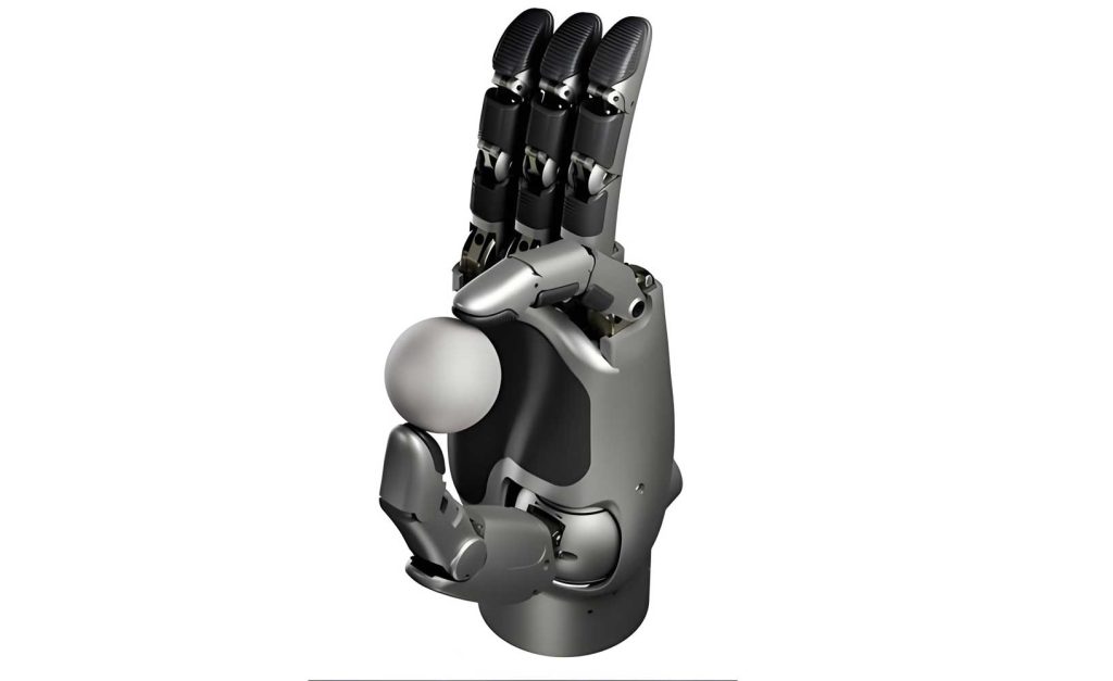
Consider a single finger segment of the dexterous robotic hand, modeled as a two-link system with a single rotary joint, as shown in Figure 1 (conceptual representation). Link 1 (the distal link) is driven relative to Link 2 (the base link) by two PAMs arranged in an antagonistic configuration within Link 2. Let \( l \) be the length of Link 1, \( m \) its mass, and \( \theta \) the joint rotation angle.
The endpoint position \((x, y)\) of Link 1 relative to the joint is given by:
$$ x = l \sin\theta $$
$$ y = l \cos\theta $$
The dynamic equation of motion for the joint is derived using the Lagrangian formulation. The Lagrangian \( L = K – P \), where \( K \) is the total kinetic energy and \( P \) is the total potential energy. For the single link rotating in a vertical plane, the equation is:
$$ \tau = \frac{1}{3} m l^2 \ddot{\theta} + c \dot{\theta} + \frac{1}{2} m g l \sin\theta $$
where \( \tau \) is the net torque applied to the joint, and \( c \) is the viscous damping coefficient of the joint.
1.2 Geometric Model of the Pneumatic Artificial Muscle
The PAM is modeled as an ideal braided mesh shell. Its geometry can be described by its length \( L \), diameter \( D \), braid angle \( \phi \) (the angle between the braided fibers and the muscle longitudinal axis), and the length of the inextensible fibers \( b \). When pressurized, the PAM contracts in length and expands in diameter, while \( b \) and the number of fiber turns \( n \) remain constant. The force \( F \) generated by the PAM as a function of contraction and internal pressure \( p \) is given by:
$$ F = \frac{p b^2}{4 \pi n^2} \left( 3 \frac{L^2}{b^2} – 1 \right) $$
This ideal geometric model relates the muscle’s force output directly to its instantaneous length and the applied pressure.
1.3 Integrated Joint Control Model
In the antagonistic setup, two PAMs (PAM1 and PAM2) act on the joint. Their length changes, \( \Delta l_1 \) and \( \Delta l_2 \), are related to the joint angle \( \theta \) through a moment arm \( R \):
$$ \theta = \frac{l_2 – l_1}{2R} = \frac{-\Delta l_1 – \Delta l_2}{2R} $$
For simplicity, we define a symmetric length variation \( \Delta l \) such that \( l_1 = l_0 + \Delta l \) and \( l_2 = l_0 – \Delta l \), where \( l_0 \) is the initial, neutral length of both PAMs. Similarly, we define pressure variations \( \Delta p \) around a common operating pressure \( p_0 \): \( p_1 = p_0 + \Delta p \) and \( p_2 = p_0 – \Delta p \). This transforms the two-input system into a single-input system with control input \( \Delta p \).
The net torque \( \tau \) generated by the antagonistic PAM pair is the difference in the forces multiplied by the moment arm:
$$ \tau = R (F_2 – F_1) $$
Substituting the geometric model force equation for each muscle and the defined symmetric variables leads to a complex nonlinear relationship between \( \Delta l \), \( \Delta p \), and \( \theta \). Combining this torque expression with the joint dynamics equation \( \tau = \frac{1}{3} m l^2 \ddot{\theta} + c \dot{\theta} + \frac{1}{2} m g l \sin\theta \) and relating \( \theta \) to \( \Delta l \) yields the full nonlinear system dynamics.
To facilitate controller design, the model is simplified through linearization. Small-angle approximation is applied to the gravitational term (\( \sin\theta \approx \theta \)), and a second-order term (\( \Delta p \cdot \Delta l \)) is neglected as a higher-order small quantity. The resulting linearized dynamic equation in terms of the length variation \( \Delta l \) is:
$$ \ddot{\Delta l} = – \frac{c}{m l^2/3} \dot{\Delta l} – \frac{3g}{2l} \Delta l + \frac{9 b^2 R}{2 \pi n^2 m l^2} \Delta p $$
We define the state variables as the length variation and its rate: \( x_1 = \Delta l \), \( x_2 = \dot{\Delta l} \). The control input is \( u = \Delta p \). The output \( y \) is the joint angle, proportional to \( x_1 \). The state-space representation of the linearized PAM-driven joint model for the dexterous robotic hand is:
$$
\begin{align*}
\dot{x}_1 &= x_2 \\
\dot{x}_2 &= -\alpha_1 x_1 – \alpha_2 x_2 + \beta u \\
y &= \gamma x_1
\end{align*}
$$
where the parameters are defined as:
$$
\alpha_1 = \frac{3g}{2l}, \quad \alpha_2 = \frac{c}{m l^2/3}, \quad \beta = \frac{9 b^2 R}{2 \pi n^2 m l^2}, \quad \gamma = -\frac{1}{R}
$$
Note that \( \alpha_1, \alpha_2, \beta \) are positive constants determined by the physical parameters of the dexterous robotic hand and the PAMs.
Design of Adaptive Joint Tracking Control
2.1 Adaptive Control Law Formulation
The linearized model parameters, particularly \( \alpha_1, \alpha_2, \) and \( \beta \), may not be known precisely or could vary slightly during operation. An adaptive control strategy is employed to ensure accurate tracking despite such uncertainties. The control objective is to make the joint angle \( y(t) \) track a desired reference signal \( r(t) \).
We define the tracking error \( e_1 = y – r = \gamma x_1 – r \). Its derivative is \( \dot{e}_1 = \gamma x_2 – \dot{r} \). We introduce a virtual control law and define a combined tracking metric \( s \), often called a sliding surface:
$$ s = \dot{e}_1 + \lambda e_1 = \gamma x_2 – \dot{r} + \lambda (\gamma x_1 – r) $$
where \( \lambda > 0 \) is a design constant. The control law is designed to drive \( s \) to zero, which guarantees convergence of the tracking error.
The derivative of \( s \) is:
$$ \dot{s} = \gamma \dot{x}_2 – \ddot{r} + \lambda (\gamma \dot{x}_1 – \dot{r}) = \gamma (-\alpha_1 x_1 – \alpha_2 x_2 + \beta u) – \ddot{r} + \lambda (\gamma x_2 – \dot{r}) $$
We design the control input \( u \) to achieve \( \dot{s} = -K s \), where \( K > 0 \), leading to exponential convergence of \( s \). The resulting control law is:
$$ u = \frac{1}{\gamma \beta} \left( \alpha_1 x_1 + \alpha_2 x_2 – \lambda (\gamma x_2 – \dot{r}) + \frac{1}{\gamma}(\ddot{r} – K s) \right) $$
Since the parameters \( \alpha_1, \alpha_2, \) and \( \beta \) are uncertain, we use their estimates \( \hat{\alpha}_1, \hat{\alpha}_2, \) and \( \hat{\beta} \) in the control law. The adaptive control law for the dexterous robotic hand joint becomes:
$$ u = \frac{1}{\gamma \hat{\beta}} \left( \hat{\alpha}_1 x_1 + \hat{\alpha}_2 x_2 – \lambda (\gamma x_2 – \dot{r}) + \frac{1}{\gamma}(\ddot{r} – K s) \right) $$
The parameter update laws are derived using Lyapunov stability theory to ensure global boundedness and convergence of the tracking error. A candidate Lyapunov function is:
$$ V = \frac{1}{2} s^2 + \frac{1}{2 \eta_1} \tilde{\alpha}_1^2 + \frac{1}{2 \eta_2} \tilde{\alpha}_2^2 + \frac{1}{2 \eta_3} \tilde{\beta}^2 $$
where \( \tilde{\alpha}_1 = \alpha_1 – \hat{\alpha}_1 \), etc., and \( \eta_i > 0 \) are adaptation gains. The time derivative \( \dot{V} \) is calculated, and the update laws are chosen to make \( \dot{V} \leq -K s^2 \), guaranteeing stability. The update laws are:
$$
\begin{align*}
\dot{\hat{\alpha}}_1 &= -\eta_1 \gamma x_1 s \\
\dot{\hat{\alpha}}_2 &= -\eta_2 \gamma x_2 s \\
\dot{\hat{\beta}} &= -\eta_3 \gamma u s
\end{align*}
$$
This completes the design of the direct adaptive tracking controller for the PAM-driven joint of the dexterous robotic hand.
2.2 Simulation Results and Comparative Analysis
The system model and controllers were implemented in Simulink for a specific set of physical parameters representative of a dexterous robotic hand finger segment. The adaptive controller was first tested for a large step command of \( 60^\circ \). The states \( x_1, x_2 \) and the parameter estimates \( \hat{\alpha}_1, \hat{\alpha}_2, \hat{\beta} \) converged rapidly to their steady-state values, demonstrating the effectiveness of the adaptation mechanism.
A comparative study was then conducted for a \( 30^\circ \) step command. The adaptive tracking controller (ATC) was compared against a well-tuned Proportional-Integral-Derivative (PID) controller. The step responses are shown in Figure 4 (conceptual).
| Performance Metric | Adaptive Tracking Control (ATC) | PID Control |
|---|---|---|
| Rise Time (s) | 0.038 | 0.211 |
| Settling Time (s) | 0.058 | 0.335 |
| Steady-State Error | Negligible | Negligible |
| Overshoot (%) | < 0.5% | ~ 2% |
The simulation results clearly indicate the superior performance of the adaptive controller. The ATC achieves a significantly faster response (approximately 5-6 times faster in terms of rise and settling times) with virtually no overshoot, compared to the PID controller. This demonstrates the advantage of the model-based adaptive approach in handling the dynamics of the PAM-actuated system within the dexterous robotic hand.
The robustness of the adaptive controller was also briefly tested by introducing a ±20% variation in the nominal values of the damping coefficient \( c \) and the PAM force constant. While the PID controller showed increased overshoot and longer settling times under these variations, the ATC maintained its performance with only minor changes in the convergence rate of parameter estimates, confirming its robustness to parameter uncertainties.
Conclusion
This work presented a comprehensive modeling and control framework for a single joint in a dexterous robotic hand actuated by pneumatic artificial muscles. By integrating the kinematic and dynamic models of the finger with the ideal geometric model of the PAMs, a nonlinear system model was developed and subsequently linearized for controller design. To address the inherent uncertainties and nonlinearities, an adaptive tracking control law was derived based on Lyapunov stability theory. The adaptive controller explicitly estimates unknown or varying system parameters online to maintain precise tracking performance.
Simulation studies confirmed the efficacy of the proposed approach. The adaptive controller demonstrated markedly superior performance compared to a conventional PID controller, offering much faster transient response, minimal overshoot, and inherent robustness to parameter variations. This validates the potential of adaptive control strategies for achieving the precise and compliant motion necessary for advanced manipulation tasks with a PAM-driven dexterous robotic hand. Future work will involve experimental validation on a physical prototype and extension of the control strategy to multi-degree-of-freedom fingers and coordinated hand control.