
The precision and reliability of the rotary vector reducer are paramount for the operational integrity of modern industrial robotics. Traditional fault diagnosis methods, often reliant on manual feature extraction from vibration signals, face significant challenges when dealing with the complex, non-linear dynamics inherent in rotary vector reducer assemblies. This paper explores a novel approach, leveraging deep learning—specifically Residual Networks (ResNet)—to automate and enhance the accuracy of fault classification for the rotary vector reducer, achieving superior performance compared to conventional neural network architectures.
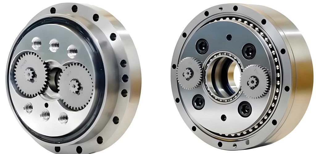
Vibration signals serve as a rich source of information regarding the mechanical health of a rotary vector reducer. However, the translation of raw, one-dimensional time-series data into actionable diagnostic insights is non-trivial. The methodology presented here begins with a structured data acquisition phase. Vibration signals are captured from a rotary vector reducer test rig under various operational loads, encompassing five distinct states: normal operation and four fault conditions, including single-component faults like planetary gear pitting and compound faults such as combined pitting on the cycloid gear and pin.
The core of our diagnostic framework is a customized Deep Residual Network. ResNets address the vanishing gradient problem common in deep networks through shortcut connections, allowing for effective training of models with many layers. For processing signals from the rotary vector reducer, the raw 1D vibration sequence of length 1024 is preprocessed into a 2D format (e.g., 32×32 matrix) via sequential stacking, making it suitable for convolutional operations. The network architecture is summarized below:
| Layer/Block Type | Configuration | Output Shape |
|---|---|---|
| Input Layer | – | (32, 32, 1) |
| Conv2D | Kernel: 7×7, Stride: 2, Filters: 64 | (16, 16, 64) |
| Max Pooling | Pool: 3×3, Stride: 2 | (8, 8, 64) |
| Residual Block 1 | [3×3 Conv, 64] x2 | (8, 8, 64) |
| Residual Block 2 | [3×3 Conv, 64] x2, Stride=2 in 1st conv | (4, 4, 64) |
| Residual Block 3 | [3×3 Conv, 128] x2 | (4, 4, 128) |
| Residual Block 4 | [3×3 Conv, 256] x2 | (4, 4, 256) |
| Global Average Pooling | – | (256) |
| Fully Connected + Softmax | 5 units | (5) |
The fundamental operation within a convolutional layer for a 2D input X with a kernel K is defined as:
$$(X * K)_{i,j} = \sum_{m} \sum_{n} X_{i-m, j-n} \cdot K_{m,n}$$
A key innovation of the ResNet is the residual block. Let the underlying mapping to be learned by a stack of layers be \( \mathcal{H}(x) \). Instead of hoping the stacked layers directly approximate \( \mathcal{H}(x) \), they are designed to approximate a residual function \( \mathcal{F}(x) = \mathcal{H}(x) – x \). The original function thus becomes \( \mathcal{H}(x) = \mathcal{F}(x) + x \). This is implemented via a shortcut connection that performs identity mapping, adding the input x to the output of the layer stack \( \mathcal{F}(x) \). This simple addition ensures that gradients can flow directly backward through the identity function, mitigating gradient vanishing. The operation within a standard residual block is:
$$\mathbf{y} = \mathcal{F}(\mathbf{x}, \{W_i\}) + \mathbf{x}$$
where \( \mathbf{x} \) and \( \mathbf{y} \) are the input and output vectors, and \( \mathcal{F}(\mathbf{x}, \{W_i\}) \) represents the residual mapping to be learned, typically involving two or three convolutional layers with weights \( W_i \).
Data preparation is critical. The collected signals are first normalized to a [0, 1] range using min-max normalization:
$$y = \frac{x – \min(x)}{\max(x) – \min(x)}$$
To augment the training dataset and improve model generalization, overlapping samples are created from the long time-series signals. If a sample has a length \( L \) and a stride \( S < L \), the number of augmented samples from a sequence of length \( M \) is approximately \( \lfloor (M – L) / S \rfloor + 1 \). This strategy significantly increases the effective size of the training set for the rotary vector reducer fault data.
The model is trained using the categorical cross-entropy loss function, which for a single sample is given by:
$$H(p, q) = -\sum_{c=1}^{C} p_c \log(q_c)$$
where \( C=5 \) is the number of fault classes, \( p \) is the true probability distribution (one-hot encoded), and \( q \) is the predicted probability distribution from the softmax output of the network. The softmax function for class \( i \) is:
$$S_i = \frac{e^{z_i}}{\sum_{j=1}^{C} e^{z_j}}$$
where \( z_i \) is the network’s output score for class \( i \).
Experimental results demonstrate the efficacy of the ResNet model for rotary vector reducer diagnosis. The model was evaluated using 5-fold cross-validation. The classification accuracy consistently surpassed that of traditional models.
| Model Architecture | Average Test Accuracy (%) | Remarks |
|---|---|---|
| Deep Neural Network (DNN) | ~63.5 | 3 Hidden Layers |
| LeNet-5 (CNN) | ~86.5 | Classical Shallow CNN |
| 10-Layer Plain CNN | ~95.7 | Without Shortcut Connections |
| Proposed ResNet | 98.11 | With Shortcut Connections |
Furthermore, the impact of different 2D reshaping configurations for the rotary vector reducer vibration signal was investigated. The results indicate that the spatial arrangement of the input matrix influences the convolutional feature extraction.
| Reshape Dimensions (Rows x Cols) | Average Accuracy (%) |
|---|---|
| 8 x 128 | 91.85 |
| 16 x 64 | 94.31 |
| 32 x 32 | 98.11 |
| 64 x 16 | 99.12 |
| 128 x 8 | 99.19 |
To validate the generalizability of the approach beyond the specific rotary vector reducer data, the same ResNet architecture was applied to the publicly available Case Western Reserve University (CWRU) bearing dataset. The model achieved an average accuracy of 99.49% on the bearing fault classification task, confirming its robustness and transferability to other rotary machinery vibration diagnostics.
An insightful analysis involves visualizing the high-dimensional features learned by the network. The 256-dimensional output from the Global Average Pooling layer, which serves as a distilled feature representation of the input rotary vector reducer signal, is projected into a 3D space using Linear Discriminant Analysis (LDA). LDA seeks a projection matrix \( W \) that maximizes the ratio of between-class scatter \( S_B \) to within-class scatter \( S_W \):
$$J(W) = \frac{W^T S_B W}{W^T S_W W}$$
Scatter plots of these 3D projections at different training stages reveal the learning progression. Initially, data points from all five rotary vector reducer conditions are intermingled. As training converges, distinct, tight clusters form for each fault class, with clear separation between them. Notably, compound fault clusters (e.g., planetary+pin pitting) show slightly more overlap with related single faults during intermediate stages, visually confirming the increased diagnostic difficulty of complex faults in the rotary vector reducer.
In conclusion, the application of Deep Residual Networks presents a powerful, data-driven solution for the fault diagnosis of the rotary vector reducer. This method eliminates the need for manual feature engineering by automatically learning hierarchical representations directly from raw vibration data. The incorporation of residual learning enables the construction of a sufficiently deep network capable of capturing the intricate patterns associated with both single and compound faults in the rotary vector reducer. The high classification accuracy, validated through rigorous cross-validation and demonstrated on an external bearing dataset, coupled with the insightful feature space visualization, underscores the potential of this deep learning framework as a reliable tool for predictive maintenance in advanced robotic systems.