
In modern industrial applications, such as robotics and precision machinery, the RV reducer plays a critical role due to its compact design, high load capacity, and superior transmission accuracy. As a novel cycloidal pinwheel transmission mechanism, the RV reducer integrates an involute planetary gear system with a cycloidal pinwheel planetary system, offering advantages like small size, light weight, large transmission ratio, and long service life. With the implementation of Industry 4.0 and initiatives like “Made in China 2025,” the demand for high-performance industrial robots has surged, emphasizing the need for precise transmission systems. However, the transmission accuracy of the RV reducer is significantly influenced by deviations arising from manufacturing and assembly processes. In this study, I analyze the deviation sources affecting the RV reducer’s performance and develop a comprehensive deviation model based on probability theory. The goal is to establish a unified framework for deviation transmission analysis, which can enhance the design and assembly of RV reducers, ultimately improving their reliability and efficiency in applications such as robotic joints and CNC machine tools.
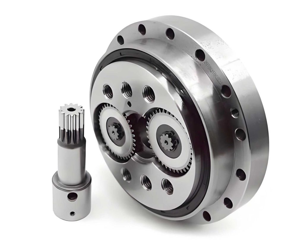
The RV reducer consists of a two-stage transmission mechanism. The first stage involves an involute planetary gear system where the sun gear meshes with planetary gears on the input shaft, providing initial speed reduction. The second stage is a cycloidal pinwheel system, where cycloidal gears engage with fixed pin gears to achieve further reduction. The structure includes components like the sun gear, planetary gears, cycloidal gears, pin gear housing, crankshafts, and the planet carrier. The transmission principle relies on the coordinated movement of these parts: when the sun gear rotates, it drives the planetary gears, which in turn rotate the crankshafts. The cycloidal gears, mounted on eccentric sections of the crankshafts, engage with the fixed pin gears, causing the planet carrier to output motion with high reduction ratios. This complex interaction makes the RV reducer susceptible to deviations that accumulate during assembly, impacting its overall transmission precision.
To address this, I classify deviation sources in the RV reducer into three categories based on their origin and impact. First, geometric position deviations (E1) refer to inaccuracies in the location and orientation of components, such as dimensional errors in crankshaft diameters or parallelism deviations between axes. These can be subdivided into positional deviations (e.g., size errors) and orientational deviations (e.g., angular misalignments). Second, geometric shape deviations (E2) involve imperfections in the form of components, such as straightness errors or profile deviations in cycloidal gear contours. Third, assembly position deviations (E3) arise from uncertainties during the fitting of parts, including gaps and misalignments due to assembly sequences. In the RV reducer, these deviations couple during assembly, leading to cumulative effects that degrade transmission accuracy. For instance, in a typical RV reducer, deviations from the crankshafts and gears can propagate through the system, causing backlash or uneven motion.
To model these deviations, I employ a vector-based approach that captures both linear and rotational aspects. Each deviation source is represented as a six-dimensional vector: $$ E_i = (\Delta u, \Delta v, \Delta w, \Delta \alpha, \Delta \beta, \Delta \gamma) $$ where $\Delta u$, $\Delta v$, and $\Delta w$ denote linear displacement deviations along the x, y, and z axes, and $\Delta \alpha$, $\Delta \beta$, and $\Delta \gamma$ represent angular deviations around these axes. The pose transformation matrix for components combines linear and rotational transformations. The linear transformation matrix is given by: $$ \text{Trans} = \begin{bmatrix} 1 & 0 & 0 & a \\ 0 & 1 & 0 & b \\ 0 & 0 & 1 & c \\ 0 & 0 & 0 & 1 \end{bmatrix} $$ where $a$, $b$, and $c$ are translations along the axes. The rotational transformation matrix is: $$ \text{Rot} = \begin{bmatrix} \cos \Delta \beta \cos \Delta \gamma & -\cos \Delta \beta \sin \Delta \gamma & \sin \Delta \beta & 0 \\ \sin \Delta \alpha \sin \Delta \beta \cos \Delta \gamma + \sin \Delta \gamma \cos \Delta \alpha & -\sin \Delta \alpha \sin \Delta \beta \sin \Delta \gamma + \cos \Delta \alpha \cos \Delta \gamma & -\sin \Delta \alpha \cos \Delta \beta & 0 \\ -\sin \Delta \alpha \sin \Delta \beta \cos \Delta \gamma + \sin \Delta \alpha \sin \Delta \gamma & \sin \Delta \beta \cos \Delta \alpha \cos \Delta \gamma + \sin \Delta \alpha \cos \Delta \gamma & \cos \Delta \alpha \cos \Delta \beta & 0 \\ 0 & 0 & 0 & 1 \end{bmatrix} $$ The overall pose transformation is then: $$ \Delta T = \text{Trans} \cdot \text{Rot} $$ This matrix encapsulates how deviations affect the position and orientation of RV reducer components during assembly.
Next, I define deviation domains to bound these errors. For geometric position deviations, domains include parallel plane zones and cylindrical zones. For example, a parallel plane deviation domain for a flat surface has limits on linear and angular deviations, as shown in the following table summarizing key parameters:
| Deviation Type | Parameters | Limits |
|---|---|---|
| Linear Deviation | $\Delta w$ | $\Delta t = t_2 – t_1$ |
| Angular Deviation | $\Delta \alpha$ | $2\Delta t / L_1$ |
| Angular Deviation | $\Delta \beta$ | $2\Delta t / W_1$ |
Here, $t_1$ and $t_2$ are tolerance limits, and $L_1$ and $W_1$ are dimensions of the plane. The constraint conditions ensure that deviations remain within acceptable ranges: $$ \Delta w + \frac{\Delta \alpha \cdot L_1}{2} \leq \Delta t $$ $$ \Delta w + \frac{\Delta \beta \cdot W_1}{2} \leq \Delta t $$ $$ \Delta w + \frac{\Delta \alpha \cdot L_1}{2} + \frac{\Delta \beta \cdot W_1}{2} \leq \Delta t $$ For cylindrical domains, similar constraints apply based on radius and length. These domains help in quantifying the maximum permissible deviations in the RV reducer’s components.
To analyze the statistical nature of deviations, I develop a multivariate statistical model assuming normal distributions for each deviation component. The linear parts follow: $$ \Delta u \sim N(\mu_1, S_1), \quad \Delta v \sim N(\mu_2, S_2), \quad \Delta w \sim N(\mu_3, S_3) $$ and the rotational parts: $$ \Delta \alpha \sim N(\mu_4, S_4), \quad \Delta \beta \sim N(\mu_5, S_5), \quad \Delta \gamma \sim N(\mu_6, S_6) $$ where $\mu_i$ are means and $S_i$ are variances. The combined model is expressed as: $$ F(E_i) = (2\pi)^{-3} (\det P)^{-1/2} e^{-\frac{1}{2} (E_i – \mu)^T P^{-1} (E_i – \mu)} $$ with mean vector $\mu = (\mu_1, \mu_2, \mu_3, \mu_4, \mu_5, \mu_6)$ and covariance matrix: $$ P = \begin{bmatrix} S_{11} & S_{12} & \cdots & S_{16} \\ S_{21} & S_{22} & \cdots & S_{26} \\ \vdots & \vdots & \ddots & \vdots \\ S_{61} & S_{62} & \cdots & S_{66} \end{bmatrix} $$ For a parallel plane deviation domain, the means and variances are derived as: $$ \mu = \left(0, 0, \frac{\max \Delta w}{2}, \frac{\max \Delta \alpha}{2}, \frac{\max \Delta \beta}{2}, 0\right) $$ $$ S_1 = 0, \quad S_2 = 0, \quad S_3 = \frac{\Delta t}{6}, \quad S_4 = \frac{\Delta t}{3L_1}, \quad S_5 = \frac{\Delta t}{3W_1}, \quad S_6 = 0 $$ This model allows for probabilistic assessment of deviation accumulation in the RV reducer.
I then evaluate each deviation source using norm-based metrics. For geometric position deviations (E1), the linear deviation magnitude is: $$ \| e(E_1) \| = \left[ (\Delta u)^2 + (\Delta v)^2 + (\Delta w)^2 + (\Delta \alpha)^2 r_\alpha^2 + (\Delta \beta)^2 r_\beta^2 + (\Delta \gamma)^2 r_\gamma^2 \right]^{1/2} $$ and the rotational deviation magnitude is: $$ \| \varepsilon(E_1) \| = \left[ \frac{(\Delta u)^2}{r_\alpha^2} + \frac{(\Delta v)^2}{r_\beta^2} + \frac{(\Delta w)^2}{r_\gamma^2} + (\Delta \alpha)^2 + (\Delta \beta)^2 + (\Delta \gamma)^2 \right]^{1/2} $$ where $r_\alpha$, $r_\beta$, and $r_\gamma$ are effective radii for angular deviations. For geometric shape deviations (E2), I first fit the component geometry to an ideal form. For a plane, the equation is: $$ F(x, y, z) = c_7 x + c_8 y + c_9 z + c_{10} = 0 $$ Using least squares fitting from measured points $O_m = (x_m, y_m, z_m)$, the fitting error is: $$ e_2 = \frac{1}{n} \sum_{m=1}^n d(O_m, F) $$ Then, the deviation magnitudes incorporate this error: $$ \| e(E_2) \| = \left[ e_2^2 + \mu_{21}^2 + \mu_{22}^2 + \mu_{23}^2 + \mu_{24}^2 r_{\alpha2}^2 + \mu_{25}^2 r_{\beta2}^2 + \mu_{26}^2 r_{\lambda2}^2 \right]^{1/2} $$ $$ \| \varepsilon(E_2) \| = \left[ \frac{e_2^2}{r_e^2} + \frac{\mu_{21}^2}{r_{\alpha2}^2} + \frac{\mu_{22}^2}{r_{\beta2}^2} + \frac{\mu_{23}^2}{r_{\lambda2}^2} + \mu_{24}^2 + \mu_{25}^2 + \mu_{26}^2 \right]^{1/2} $$ For assembly position deviations (E3), similar expressions apply: $$ \| e(E_3) \| = \left[ \mu_{31}^2 + \mu_{32}^2 + \mu_{33}^2 + \mu_{34}^2 r_{\alpha3}^2 + \mu_{35}^2 r_{\beta3}^2 + \mu_{36}^2 r_{\lambda3}^2 \right]^{1/2} $$ $$ \| \varepsilon(E_3) \| = \left[ \frac{\mu_{31}^2}{r_{\alpha3}^2} + \frac{\mu_{32}^2}{r_{\beta3}^2} + \frac{\mu_{33}^2}{r_{\lambda3}^2} + \mu_{34}^2 + \mu_{35}^2 + \mu_{36}^2 \right]^{1/2} $$ The total deviation for a component combines these sources: linear deviation $d_1 = \| e(E_1) \| + \| e(E_2) \| + \| e(E_3) \|$ and rotational deviation $\psi_1 = \| \varepsilon(E_1) \| + \| \varepsilon(E_2) \| + \| \varepsilon(E_3) \|$.
To understand how deviations propagate in the RV reducer, I analyze the transmission mechanism using directed graphs. Deviation sources are represented as nodes, and their interactions as edges. Basic deviation flows include: $f_1$ for intra-component geometric position deviations, $f_2$ for shape deviations, $f_3$ for inter-component geometric deviations, $f_4$ for assembly position deviations (as corrections), and $f_5$ for multiple coupled deviations. The directed graph helps visualize how errors accumulate through the assembly sequence. For instance, in the RV reducer, deviations from the sun gear may affect planetary gears, then crankshafts, and finally the cycloidal gears, leading to output inaccuracies.
Deviation transmission occurs via two primary modes: continuous flow ($f_a$) through geometric constraints in non-clearance fits, and discontinuous flow ($f_b$) through positional uncertainties in clearance fits. The RV reducer’s配合 relationships are categorized into three types: Mgg (both geometries are deviation-prone), MDD (both are datum geometries), and MgD (mixed). In non-clearance fits (Mf), deviations transfer continuously as one component’s inaccuracy forces another out of position. In clearance fits (Mc), gaps interrupt the flow, and assembly position deviations dominate. The table below summarizes these relationships:
| Fit Type | Description | Deviation Flow |
|---|---|---|
| Mgg (Mf) | Non-clearance, both geometries deviated | Continuous ($f_a$) |
| Mgg (Mc) | Clearance, both geometries deviated | Discontinuous ($f_b$) |
| MgD (Mc) | Clearance, mixed geometries | Discontinuous with corrections |
For example, in an Mgg-type clearance fit, the deviation vector is $E = \Delta T_2 + \Delta d_2$, where $\Delta T_2$ is the assembly position deviation and $\Delta d_2$ is the geometric deviation. This model allows for precise tracking of error paths in the RV reducer assembly.
To validate the deviation model, I consider a practical case of shaft-hole fitting in an RV reducer component. Assume a shaft (part 1) with diameter $d_1 = 25^{+0.1}_{0}$ mm and a hole (part 2) with diameter $d_2 = 25^{0}_{-0.15}$ mm, forming a clearance fit. Using the multivariate deviation vector model, I calculate the total deviations. Based on extreme value analysis, the linear total deviation is: $$ d_1 = 0.4970 \, \text{mm} $$ and the rotational total deviation is: $$ \psi_1 = 0.0269 \, \text{mm} $$ Using trigonometric similarity, the angular deviation is $\Delta \theta = 0.0573^\circ$. This result aligns with ideal tolerances, showing a difference within $0.11^\circ$, which meets assembly quality requirements for the RV reducer. This example demonstrates how the model can predict deviation effects in real-world scenarios, aiding in the design of more precise RV reducers.
In conclusion, this study provides a comprehensive framework for analyzing deviations in RV reducers. By classifying deviation sources into geometric position, shape, and assembly position categories, I establish a unified model that integrates vector representations, statistical distributions, and deviation domains. The directed graph approach elucidates transmission mechanisms, highlighting how errors propagate through different fit types. The instance of shaft-hole fitting confirms the model’s accuracy, with deviations calculated within acceptable limits. This work not only enhances understanding of RV reducer precision but also offers a methodology applicable to other mechanical assemblies. Future research could extend this model to dynamic conditions or integrate it with optimization algorithms for tolerance design, further advancing the reliability of RV reducers in high-precision industries.