
In the pursuit of high-precision, compact, and high-torque transmission systems, one technology stands out for its unique operating principle and exceptional performance characteristics: the strain wave gear, commonly known as the harmonic drive. This research delves into the intricate optimization challenges inherent in the design of strain wave gear systems. Traditional optimization methods, often constrained by assumptions of design variable continuity, yield results that are impractical for direct manufacturing. Parameters such as gear module, which must align with standardized discrete values, or tooth counts, which are inherently integer-based, render purely continuous-variable solutions merely theoretical. To bridge this gap between optimal theory and manufacturable reality, this article proposes a novel approach: a hybrid discrete variable fuzzy optimization model solved by an enhanced Ant Colony Algorithm (ACA). This methodology rigorously accounts for the mixed-integer nature of the design problem while incorporating the inherent fuzziness of engineering constraints, culminating in a design process that is both mathematically sound and immediately applicable on the shop floor.
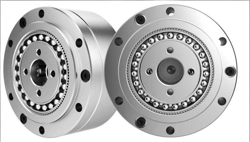
The fundamental advantage of a strain wave gear lies in its revolutionary design, which forgoes rigid gear meshing in favor of elastic deformation. A typical configuration comprises three core components: a rigid circular spline (the “ring gear”), a flexible spline (the “flexspline”), and a wave generator. The wave generator, often an elliptical bearing assembly, is inserted into the flexspline, causing it to deform into an elliptical shape. This deformation engages the teeth of the flexspline with those of the circular spline at two opposing regions. As the wave generator rotates, the points of engagement travel around the gear circumference. Critically, the flexspline has slightly fewer teeth (typically 2 teeth fewer for a standard “cup” type) than the circular spline. This difference in tooth count means that for every full revolution of the wave generator, the flexspline rotates backward relative to the circular spline by a small amount equal to the tooth differential. This kinematic relationship yields remarkably high reduction ratios in a single stage, given by:
$$
i = -\frac{z_g}{z_g – z_f}
$$
where $z_g$ is the number of teeth on the circular spline and $z_f$ is the number of teeth on the flexspline. The negative sign indicates the reversal in the direction of rotation.
The compactness, near-zero backlash, high torque capacity, and coaxial input/output configuration make the strain wave gear indispensable in fields like aerospace robotics, precision optical positioning systems, and medical devices. However, this performance comes at the cost of complexity. The flexspline undergoes high-cycle elastic deformation, making its fatigue life a primary design constraint. The unique tooth geometry and meshing kinematics introduce constraints to prevent interference. Therefore, the design of a strain wave gear is a tightly coupled, nonlinear, constrained optimization problem where the goal is to minimize volume (and thus weight and material cost) while ensuring structural integrity and kinematic functionality.
The Mathematical Model for Strain Wave Gear Optimization
Formulating a precise optimization model is the first critical step. We consider a standard single-stage reducer with a cup-type flexspline, a rigid circular spline, and a dual-wave (“four-contact-point”) generator. The primary goal is to minimize the total volume of the gear set, which serves as a direct proxy for minimizing weight and material usage.
Design Variables and Objective Function
The design is governed by a set of six key parameters, forming our design variable vector:
$$
\mathbf{x} = [z_g, z_f, m, L, b, h_2]^T = [x_1, x_2, x_3, x_4, x_5, x_6]^T
$$
Their nature and significance are outlined below:
| Variable | Symbol | Description | Type |
|---|---|---|---|
| $x_1$ | $z_g$ | Number of teeth on the circular spline | Integer |
| $x_2$ | $z_f$ | Number of teeth on the flexspline | Integer |
| $x_3$ | $m$ | Gear module (standardized value) | Non-uniform discrete |
| $x_4$ | $L$ | Length of the flexspline cup | Integer |
| $x_5$ | $b$ | Face width of the gears | Integer |
| $x_6$ | $h_2$ | Nominal wall thickness of the flexspline cup | Continuous (to 0.1mm) |
The objective function representing the approximate total volume $f(\mathbf{x})$ is derived from the geometries of the flexspline cup and the circular spline ring:
$$
f(\mathbf{x}) = \pi L h_2 \left( \frac{d_{f2}}{2} – h_1 + \frac{h_2}{2} \right)^2 + \frac{\pi}{4} b (h_{gf} + S_g) d_g^2
$$
where:
- $d_{f2}$ is the root diameter of the flexspline: $d_{f2} = z_f m – \frac{9}{4}m$.
- $h_1$ is the wall thickness at the flexspline tooth root, typically set as $h_1 = 2h_2$.
- $d_g$ is the pitch diameter of the circular spline: $d_g = z_g m$.
- $h_{gf}$ is the tooth height of the circular spline, taken as $2m$.
- $S_g$ is the rim thickness of the circular spline, taken as $20m$.
Substituting these relationships, the objective function simplifies to a form explicitly in terms of the design variables:
$$
f(\mathbf{x}) = \pi L h_2 \left( \frac{z_f m}{2} – \frac{9}{8}m – 1.5h_2 \right)^2 + 5.5 \pi b m^3 z_g^2
$$
This clearly shows the coupling between variables and the primary goal of minimizing this composite volume.
Fuzzy and Deterministic Constraint Formulation
The feasibility of a design is enforced by a set of constraints that are both deterministic and fuzzy in nature.
1. Flexspline Fatigue Strength (Fuzzy Constraint): The flexspline is subjected to complex, alternating stresses. Its safety factor against fatigue failure must be sufficient. However, the required safety factor is not a crisp number; it is a fuzzy concept where values slightly above 1.5 are fully acceptable, and values slightly below are increasingly unacceptable. The combined stress safety factor $S$ is calculated based on von Mises criteria for alternating stresses:
$$
S = \frac{S_{-1}}{\sqrt{\sigma_a^2 + (K_\tau \tau_a)^2}} \gtrsim 1.5
$$
where $S_{-1}$ is the fatigue limit of the flexspline material in fully reversed bending, $\sigma_a$ and $\tau_a$ are the alternating bending and shear stress amplitudes, and $K_\tau$ is a stress concentration factor. The symbol $\gtrsim$ denotes “fuzzily greater than or equal to.” This fuzzy constraint is later resolved using an optimal cut-level $\lambda^*$ derived from fuzzy comprehensive evaluation, transforming it into an ordinary inequality: $S \geq 1.5 – (1-\lambda^*)d$, where $d$ is a tolerance parameter.
2. Kinematic Non-Interference Constraint: To ensure smooth meshing without tooth tip interference between the circular spline and flexspline during engagement and disengagement, a specific kinematic condition must be met. This involves comparing the rotation angles corresponding to the working tooth profiles:
$$
\theta_{g1} – \theta_{f1} \geq 0
$$
The detailed calculation of $\theta_{g1}$ and $\theta_{f1}$ depends on the tooth geometry, deformation function of the wave generator, and the initial phase of engagement.
3. Transmission Ratio Constraint (Equality): The design must achieve a specified reduction ratio $i$. This introduces an equality constraint:
$$
i – \frac{z_g}{z_g – z_f} = 0 \quad \text{or equivalently} \quad i(z_g – z_f) – z_f = 0
$$
This constraint strictly couples the two integer variables $z_g$ and $z_f$.
4. Boundary and Empirical Constraints: Based on design manuals and empirical data, practical limits are placed on geometric proportions:
$$
\begin{aligned}
&0.1 d_f \leq L \leq 0.2 d_f \\
&0.15 d_f \leq b \leq 0.25 d_f \\
&0.010 d_f \leq h_2 \leq 0.015 d_f \\
&180 \leq z_g \leq 230 \\
&178 \leq z_f \leq 228 \quad \text{(with } z_g – z_f = 2\text{)}
\end{aligned}
$$
Here, $d_f = z_f m$ is the pitch diameter of the flexspline. These constraints ensure manufacturability and adherence to established design principles for strain wave gear systems.
The complete model is thus a Mixed-Integer Non-Linear Programming (MINLP) problem with both equality and inequality constraints, a challenge for conventional gradient-based optimizers.
Principles and Enhancement of the Ant Colony Algorithm
Inspired by the foraging behavior of real ants, the Ant Colony Algorithm is a population-based metaheuristic perfectly suited for combinatorial optimization problems. Ants find the shortest path to food by depositing pheromones. Paths with higher pheromone concentration attract more ants, creating a positive feedback loop that converges on the optimal route. We transpose this metaphor to our design space.
Core ACA Mechanics for Optimization
In our virtual setting, each ant represents a candidate design vector $\mathbf{x}^k$. The “path length” is analogous to the objective function value $f(\mathbf{x}^k)$; a lower volume signifies a shorter, better path. The algorithm proceeds in iterative cycles with two main phases:
1. Local Search and Probabilistic Transition: Each ant performs a local search within a shrinking neighborhood radius $R^{t+1} = \eta R^t$ ($0<\eta<1$). Subsequently, an ant $i$ may decide to “jump” to the position of another ant $j$ with a probability $p_{ij}$. This probability balances the attraction of good solutions (pheromone intensity $\tau_j$) and their relative improvement (heuristic information $\eta_{ij}$):
$$
p_{ij} = \frac{[\tau_j]^\alpha [\eta_{ij}]^\beta}{\sum_{l \in \mathcal{J}} [\tau_l]^\alpha [\eta_{il}]^\beta}, \quad \forall j \in \mathcal{J}
$$
where $\mathcal{J}$ is the set of reachable ants (often all others), and $\alpha$ and $\beta$ control the relative influence of pheromone versus heuristic. The heuristic desirability $\eta_{ij}$ is defined as the perceived gain in moving from a worse solution $i$ to a better one $j$:
$$
\eta_{ij} = \max(0, f(\mathbf{x}^i) – f(\mathbf{x}^j))
$$
If $f(\mathbf{x}^j)$ is not better, $\eta_{ij}=0$, making a jump unlikely.
2. Pheromone Update: After all ants have completed their moves, the pheromone trails are updated. This involves both evaporation (to forget poor paths) and deposition (to reinforce good ones):
$$
\tau_j^{\,new} = \rho \cdot \tau_j^{\,old} + \sum_{k=1}^{m} \Delta \tau_j^k
$$
where $\rho \in (0, 1)$ is the evaporation rate, and $\Delta \tau_j^k$ is the amount of pheromone ant $k$ deposits on path $j$. Typically, $\Delta \tau_j^k = Q / f(\mathbf{x}^j)$ if ant $k$ visited solution $j$, and $0$ otherwise, with $Q$ being a constant. This ensures better solutions receive stronger reinforcement.
Algorithmic Enhancements for Engineering Design
The canonical ACA has limitations, notably the potential for premature convergence to a local optimum. Furthermore, it is not natively equipped to handle mixed discrete variables or constrained problems. We introduce three key enhancements.
1. Anti-Premature Convergence Mechanism: To prevent the colony from stagnating, we monitor convergence health every $P$ iterations (e.g., $P=8$). We trigger a colony renewal if two conditions hold simultaneously:
$$
\left\{ \left(f_{min}^{(t-P)} – f_{min}^{(t)}\right) = 0 \right\} \bigcap \left\{ \left( \frac{f_{mean}^{(t)} – f_{min}^{(t)}}{f_{mean}^{(t)}} \right) < \epsilon \right\}
$$
where $f_{min}$ and $f_{mean}$ are the best and average objective values in the colony, and $\epsilon$ is a small threshold (e.g., 0.02). The first condition checks if the global best has not improved in $P$ cycles. The second checks if the colony’s diversity is too low (all ants are clustered near the best). If triggered, the best ant is preserved (elitism), and the rest of the colony is reinitialized randomly, injecting new exploration potential.
2. Engineering Discretization During Search: This is the crucial step for handling mixed variables. During every function evaluation, the ant’s raw position vector $\mathbf{x}_{raw}$ is mapped to an engineering-feasible vector $\mathbf{x}_{eng}$ before calculating $f(\mathbf{x})$ or constraints:
- Integer variables ($z_g, z_f, L, b$): $\mathbf{x}_{eng}[i] = \text{round}(\mathbf{x}_{raw}[i])$.
- Standard Module ($m$): $\mathbf{x}_{eng}[m] = \text{argmin}( |\mathbf{x}_{raw}[m] – M_i| )$ where $M_i \in \{0.25, 0.3, 0.4, …, 1.0, 1.25, …\}$ (standard series).
- Continuous Variable ($h_2$): $\mathbf{x}_{eng}[h_2] = \text{round}( \mathbf{x}_{raw}[h_2], 1)$ (to one decimal place).
The ants effectively search the discretized space, ensuring every evaluated solution is directly manufacturable.
3. Constraint Handling via Penalty Function: The ACA core operates on unconstrained problems. We employ an exterior penalty function method to convert the constrained problem into an unconstrained one. The modified objective function $F(\mathbf{x})$ for the algorithm is:
$$
F(\mathbf{x}) = f(\mathbf{x}_{eng}) + \mu \sum_{q=1}^{r} \left[ \max(0, g_q(\mathbf{x}_{eng})) \right]^2 + \nu \cdot (h(\mathbf{x}_{eng}))^2
$$
where $g_q$ are inequality constraints, $h$ is the equality constraint (transmission ratio), and $\mu$ and $\nu$ are large, iteratively increasing penalty factors. This strongly penalizes infeasible ants, guiding the search towards the feasible region.
Implementation and Optimization Case Study
The enhanced Hybrid Discrete Ant Colony Algorithm (HD-ACA) was implemented in a computational framework using MATLAB, resulting in the program `Ls_Antalg`. The program’s workflow is summarized in the following pseudocode:
| Step | Action |
|---|---|
| 1 | Initialize: Set algorithm parameters (colony size $m$, max iterations $T_{max}$, $\alpha$, $\beta$, $\rho$, $\eta$, $P$, $\epsilon$). |
| 2 | Generate Colony: Randomly create $m$ initial ant positions within bounds. |
| 3 | Evaluate & Discretize: For each ant, apply engineering discretization and calculate penalized objective $F(\mathbf{x})$. |
| 4 | Pheromone Init: Initialize pheromone trails $\tau_j$ (e.g., to 1). |
| 5 | While $t < T_{max}$ do |
| 6 | Local Search: Each ant explores its discretized neighborhood. |
| 7 | Probabilistic Jump: Each ant may jump to another ant’s position based on $p_{ij}$. |
| 8 | Update Pheromones: Apply evaporation and deposition per Eq. (7). |
| 9 | Check Convergence: If (iteration mod $P$ == 0) and Eq. (8) is true, preserve best ant and reinitialize the rest. |
| 10 | $t = t + 1$ |
| 11 | End While |
| 12 | Output: Return the best-found feasible design $\mathbf{x}^*$ and $f(\mathbf{x}^*)$. |
Design Specification and Fuzzy Constraint Processing
We consider a strain wave gear reducer with the following requirements:
- Transmission Ratio ($i$): 100
- Output Torque: 500 Nm
- Input Speed: 3000 rpm
- Duty Cycle: 8-10 hours/day, smooth operation.
- Flexspline Material: 40CrNiMoA, with fatigue limits $\sigma_{-1}=500$ MPa, $\tau_{-1}=250$ MPa.
The fuzzy strength constraint was processed using the expansion coefficient method combined with fuzzy comprehensive evaluation. An optimal cut-level $\lambda^* = 0.91$ was determined, transforming the fuzzy safety factor requirement $S \gtrsim 1.5$ into the deterministic constraint $S \geq 1.45$.
Optimization Results and Comparative Analysis
The HD-ACA was executed with a colony size of $m=20$ and a maximum of 300 iterations. The algorithm consistently converged to an optimal, manufacturable design. The results are compared below with those from other optimization methods applied to the same problem, highlighting the practical advantage of the discrete-variable approach.
| Optimization Method | $z_g$ | $z_f$ | $m$ (mm) | $L$ (mm) | $b$ (mm) | $h_2$ (mm) | $f(\mathbf{x})$ (mm³) | Major Iterations |
|---|---|---|---|---|---|---|---|---|
| Proposed HD-ACA | 202 | 200 | 0.5 | 120 | 20 | 1.0 | 2,628,933.3 | ~250 |
| Hybrid Discrete GA (Reference) | 202 | 200 | 0.5 | 120 | 20 | 1.0 | 2,628,933.3 | >400 |
| Continuous Variable Method (e.g., Chaos GA) | 187.417 | 185.562 | 0.539 | 120.065 | 20.035 | 1.002 | 2,775,199.1 | >450 |
The analysis reveals critical insights:
- Manufacturability: The proposed HD-ACA and the reference discrete GA yield identical, directly usable parameters. The module is a standard 0.5 mm, and all dimensions are clean, rational numbers. The continuous method produces irrational numbers (e.g., module 0.539 mm, 185.562 teeth), which are impossible to manufacture without violating the problem’s fundamental discrete nature. Simple rounding of these values could lead to constraint violation or loss of optimality.
- Performance: The volume found by the discrete methods is approximately 5.3% lower than that from the rounded continuous solution, demonstrating that forcing continuity can lead to a physically inferior design point.
- Efficiency: While matching the result of a sophisticated Hybrid Discrete GA, the enhanced ACA required significantly fewer major iterations (around 250 vs. over 400) to locate the global optimum, indicating its strong search capability and convergence speed for this class of MINLP problems.
Conclusion
This research successfully addresses the complex, mixed-integer nature of strain wave gear design optimization. By formulating a fuzzy optimization model that incorporates the imprecision of engineering judgments and the hard realities of manufacturing standards, and by employing a robustly enhanced Ant Colony Algorithm to solve it, we bridge a critical gap between theoretical optimization and practical engineering. The key innovations—the anti-premature convergence mechanism and the in-search engineering discretization—ensure the algorithm efficiently explores the feasible, discrete design space, avoiding the pitfalls of local optima and delivering solutions that require no post-processing. The case study unequivocally demonstrates that methodologies which respect the discrete nature of design variables yield superior, immediately implementable results compared to those based on continuous relaxation. The proposed HD-ACA framework is not limited to strain wave gear optimization; it is readily adaptable to a wide array of mechanical design problems characterized by mixed discrete variables, nonlinear constraints, and complex objective landscapes, offering a powerful tool for designers seeking truly optimal and practical solutions.