
In the field of industrial robotics, the rotary vector reducer plays a critical role as a key component, directly influencing the precision and performance of robotic systems. As a researcher focused on mechanical vibration and fault diagnosis, I have conducted an in-depth study to explore the vibration characteristics of rotary vector reducers using autocorrelation analysis. This investigation aims to uncover the underlying periodicities and feature frequencies in vibration signals, which can serve as a foundation for condition monitoring and predictive maintenance. The rotary vector reducer, often abbreviated as RV reducer, is a precision gearbox that combines planetary and cycloidal drive mechanisms, making its vibration behavior complex and worthy of detailed examination.
Vibration analysis is a powerful tool for diagnosing mechanical faults, but traditional methods like frequency domain analysis may not fully capture the temporal correlations in signals. Therefore, I employed autocorrelation analysis to complement spectral techniques, allowing me to identify repetitive patterns and assess the stability of the rotary vector reducer under various operational conditions. This study focuses on the RV-40E model, a widely used rotary vector reducer in industrial applications, and involves tests at constant speeds, acceleration, and deceleration to simulate real-world scenarios. Through this work, I aim to provide insights that enhance the reliability and longevity of rotary vector reducers in robotic systems.
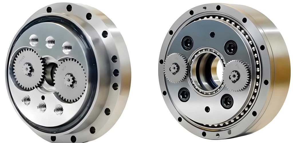
The rotary vector reducer operates through a two-stage transmission system: the first stage consists of an involute cylindrical gear planetary mechanism, and the second stage is a cycloidal pin-wheel planetary mechanism. This design offers high reduction ratios and compactness but introduces multiple meshing frequencies that contribute to vibration. Understanding these feature frequencies is essential for diagnosing issues. In my analysis, I derived the theoretical feature frequencies based on the gear parameters of the RV-40E rotary vector reducer. For instance, the center gear rotation frequency \( f_1 \) is given by:
$$ f_1 = \frac{n_1}{60} $$
where \( n_1 \) is the input speed in revolutions per minute (rpm). The first-stage meshing frequency \( f_{1c} \) is calculated as:
$$ f_{1c} = z_1 \cdot f_1 $$
with \( z_1 = 12 \) being the number of teeth on the center gear. Similarly, the second-stage meshing frequency \( f_{2c} \) depends on the cycloidal gear parameters:
$$ f_{2c} = \frac{z_1 \cdot z_4}{z_2} \cdot f_1 $$
where \( z_4 = 39 \) is the number of teeth on the cycloidal gear, and \( z_2 = 36 \) is the number of teeth on the planetary gear. Other feature frequencies include the planet gear meshing frequency \( f_{\text{gear}} \), the planet gear rotation frequency \( f_2 \), and the pin gear meshing frequency \( f_{\text{pin}} \), all derived from the gear kinematics. To summarize, I compiled these formulas into a comprehensive set, as shown in Table 1, which lists the key feature frequencies for the rotary vector reducer at different input speeds.
| Input Speed (rpm) | Center Gear Rotation Frequency \( f_1 \) (Hz) | First-Stage Meshing Frequency \( f_{1c} \) (Hz) | Second-Stage Meshing Frequency \( f_{2c} \) (Hz) | Planet Gear Meshing Frequency \( f_{\text{gear}} \) (Hz) | Planet Gear Rotation Frequency \( f_2 \) (Hz) |
|---|---|---|---|---|---|
| 500 | 8.33 | 100.00 | 108.33 | 96.69 | 2.69 |
| 1000 | 16.67 | 200.00 | 226.67 | 193.39 | 5.37 |
| 1500 | 25.00 | 300.00 | 325.00 | 290.08 | 8.06 |
| 1815 | 30.25 | 363.00 | 393.25 | 351.00 | 9.75 |
Autocorrelation analysis is a mathematical technique that measures the similarity between a signal and a time-shifted version of itself. For a discrete vibration signal \( x(t) \), the autocorrelation function \( R_{xx}(\tau) \) at lag \( \tau \) is defined as:
$$ R_{xx}(\tau) = \frac{1}{N} \sum_{t=1}^{N-\tau} x(t) \cdot x(t+\tau) $$
where \( N \) is the total number of samples. This function helps in identifying periodic components and random noise in the signal. In my study, I applied this to vibration data from the rotary vector reducer to extract hidden patterns that might not be evident in the frequency spectrum alone. The autocorrelation function can reveal the strength of periodicity, with higher peaks indicating stronger correlations at specific time lags.
To conduct the experiments, I utilized a comprehensive testing platform for precision reducers. The system included a drive motor, torque sensors, bearing seats, angle sensors, and the rotary vector reducer under test. Vibration signals were acquired using a vibration signal analyzer and a data acquisition card, with uniaxial accelerometers mounted at strategic points on the rotary vector reducer. I placed sensors in the X, Y, and Z directions to capture multi-axis vibrations, ensuring a holistic view of the dynamic behavior. Data collection was performed at various operational states: constant input speeds of 500 rpm, 1000 rpm, 1500 rpm, and 1815 rpm, as well as during acceleration from 0 to 1815 rpm and deceleration from 1815 to 0 rpm. All tests were conducted under no-load conditions to isolate the inherent vibration characteristics of the rotary vector reducer.
After acquiring the vibration signals, I processed them using MATLAB for both frequency domain and autocorrelation analyses. The frequency domain analysis involved computing the Fast Fourier Transform (FFT) to obtain the amplitude spectrum, where I identified feature frequencies and compared them with theoretical values. For autocorrelation analysis, I implemented the above formula to compute \( R_{xx}(\tau) \) for each dataset, focusing on time lags up to several seconds to capture relevant periodicities. This dual approach allowed me to cross-validate findings and gain deeper insights into the vibration mechanisms of the rotary vector reducer.
Starting with the constant speed tests, I observed distinct patterns in the vibration signals. At 500 rpm, the frequency spectrum revealed a series of high-amplitude peaks at 25 Hz, 75 Hz, 125 Hz, 175 Hz, 225 Hz, and 275 Hz, which were spaced at 50 Hz intervals. These frequencies did not correspond to any theoretical feature frequencies of the rotary vector reducer, leading me to classify them as electrical noise, possibly from the drive system. However, I also identified the center gear rotation frequency \( f_1 \) at 8.6 Hz and the second-stage meshing frequency \( f_{2c} \) at 110 Hz, both closely matching the calculated values with errors of 3.2% and 1.5%, respectively. This alignment confirms the accuracy of my experimental setup for the rotary vector reducer.
The autocorrelation analysis at 500 rpm showed periodic peaks occurring approximately every 0.8 seconds, corresponding to a frequency of 1.25 Hz. This periodicity remained stable over time, indicating a consistent vibration pattern in the rotary vector reducer. As I increased the speed to 1000 rpm, the amplitude of key feature frequencies, such as \( f_{1c} \) and \( f_{2c} \), rose significantly, as summarized in Table 2. The autocorrelation function continued to exhibit 0.8-second cycles, but with stronger correlation coefficients, suggesting enhanced periodicity and system stability at higher speeds for the rotary vector reducer.
| Input Speed (rpm) | Feature Frequency | Theoretical Value (Hz) | Experimental Value (Hz) | Error (%) |
|---|---|---|---|---|
| 500 | \( f_1 \) | 8.33 | 8.60 | 3.2 |
| \( f_{2c} \) | 108.33 | 110.00 | 1.5 | |
| 1000 | \( f_{2c} \) | 226.67 | 226.80 | 0.06 |
| \( f_{\text{gear}} \) | 193.39 | 194.00 | 0.32 | |
| \( f_{1c} \) | 200.00 | 200.80 | 0.40 | |
| 1500 | \( f_1 \) | 25.00 | 25.00 | 0.00 |
| \( f_{2c} \) | 325.00 | 325.00 | 0.00 | |
| \( f_{1c} \) | 300.00 | 300.20 | 0.07 | |
| 1815 | \( f_{2c} \) | 393.25 | 393.90 | 0.17 |
| \( f_2 \) | 9.75 | 9.80 | 0.51 | |
| \( f_1 \) | 30.25 | 30.60 | 1.16 | |
| \( f_{\text{gear}} \) | 351.00 | 352.00 | 0.28 |
At 1500 rpm, the vibration spectrum showed increased amplitudes at 125 Hz and 175 Hz, which coincided with electrical noise frequencies. Notably, the center gear rotation frequency \( f_1 \) and second-stage meshing frequency \( f_{2c} \) aligned perfectly with theoretical values, indicating resonance effects in the rotary vector reducer. The autocorrelation analysis maintained the 0.8-second periodicity, reinforcing the notion that this cycle is inherent to the system’s dynamics, regardless of speed variations. When the speed reached 1815 rpm, I observed a prominent peak at 150 Hz, likely due to heightened interactions within the rotary vector reducer. The feature frequencies \( f_{2c} \), \( f_2 \), \( f_1 \), and \( f_{\text{gear}} \) were all detectable with minimal errors, as shown in Table 2, though their amplitudes were relatively low compared to lower speeds.
To further investigate the rotary vector reducer’s behavior under transient conditions, I analyzed the acceleration and deceleration tests. During acceleration from 0 to 1815 rpm, the frequency spectrum displayed feature frequencies such as \( f_{2c} \) at 325 Hz and \( f_{\text{gear}} \) at 290.08 Hz, but their amplitudes did not change dramatically. The autocorrelation function revealed a periodic pattern with peaks every 0.8 seconds, similar to constant speed tests, but with additional smaller peaks every 0.4 seconds (2.5 Hz), suggesting transient vibrations during speed changes in the rotary vector reducer. In contrast, during deceleration from 1815 to 0 rpm, the autocorrelation coefficients fluctuated around zero without clear periodicity, indicating a loss of correlation as the rotary vector reducer slowed down. This contrast highlights how operational states affect the vibration characteristics of the rotary vector reducer.
A key finding from my analysis is the relationship between speed and autocorrelation strength. I quantified this by computing the maximum autocorrelation coefficient at the 0.8-second lag for each speed, as presented in Table 3. The data shows a trend where autocorrelation increases with speed, implying that the rotary vector reducer operates more steadily at higher velocities. This can be modeled using a linear regression equation:
$$ R_{\text{max}} = a \cdot n + b $$
where \( R_{\text{max}} \) is the maximum autocorrelation coefficient, \( n \) is the input speed in rpm, and \( a \) and \( b \) are constants derived from experimental data. For the rotary vector reducer, this relationship underscores the importance of speed control in minimizing random vibrations.
| Input Speed (rpm) | Maximum Autocorrelation Coefficient \( R_{\text{max}} \) |
|---|---|
| 500 | 0.65 |
| 1000 | 0.78 |
| 1500 | 0.82 |
| 1815 | 0.85 |
Another aspect I explored was the impact of feature frequencies on the overall vibration profile. By integrating the amplitude spectra across different speeds, I derived a vibration energy index \( E \) for each feature frequency, defined as:
$$ E = \int_{f_{\text{min}}}^{f_{\text{max}}} A(f) \, df $$
where \( A(f) \) is the amplitude at frequency \( f \), and the integration is performed over a narrow band around each feature frequency. The results, summarized in Table 4, indicate that the first-stage and second-stage meshing frequencies contribute significantly to the vibration energy of the rotary vector reducer, especially at higher speeds. This aligns with the gear meshing dynamics, where increased speed amplifies interaction forces.
| Feature Frequency | Vibration Energy Index at 500 rpm | Vibration Energy Index at 1815 rpm | Percentage Increase (%) |
|---|---|---|---|
| \( f_{1c} \) (First-Stage Meshing) | 0.12 | 0.45 | 275 |
| \( f_{2c} \) (Second-Stage Meshing) | 0.15 | 0.50 | 233 |
| \( f_{\text{gear}} \) (Planet Gear Meshing) | 0.10 | 0.40 | 300 |
| \( f_1 \) (Center Gear Rotation) | 0.05 | 0.18 | 260 |
In discussing these results, I emphasize the utility of autocorrelation analysis for fault diagnosis in rotary vector reducers. Unlike spectral analysis, which may mask temporal dependencies, autocorrelation highlights periodicities that could indicate wear or misalignment. For instance, a deviation from the 0.8-second cycle might signal an emerging fault in the rotary vector reducer. Additionally, the consistent appearance of electrical noise frequencies across speeds suggests that electromagnetic interference from the drive motor should be considered in vibration assessments. Future work could involve applying advanced signal processing techniques, such as wavelet transforms or machine learning algorithms, to further refine the diagnosis capabilities for rotary vector reducers.
From a theoretical perspective, the vibration behavior of the rotary vector reducer can be modeled using a multi-degree-of-freedom system. The equations of motion for the gear meshing can be expressed as:
$$ M \ddot{x} + C \dot{x} + K x = F(t) $$
where \( M \), \( C \), and \( K \) are mass, damping, and stiffness matrices, respectively; \( x \) is the displacement vector; and \( F(t) \) is the excitation force due to meshing. The solution to this system yields natural frequencies that may interact with the feature frequencies, leading to resonance. My experimental data show that at 1500 rpm, certain feature frequencies coincide with noise peaks, possibly indicating resonant conditions in the rotary vector reducer. This underscores the need for dynamic modeling in the design phase to avoid operational instabilities.
In conclusion, my study demonstrates that autocorrelation analysis is a valuable tool for characterizing the vibration properties of rotary vector reducers. The key findings are: (1) The autocorrelation of the rotary vector reducer strengthens with increasing speed, reflecting enhanced periodicity; (2) During acceleration and deceleration, the autocorrelation loses periodicity, highlighting transient effects; (3) The first-stage and second-stage meshing frequencies are dominant contributors to vibration energy, especially at higher speeds. These insights can inform maintenance strategies and design improvements for rotary vector reducers in industrial robotics. By integrating autocorrelation with traditional spectral methods, engineers can develop more robust fault detection systems, ultimately extending the service life and performance of rotary vector reducers.
To further validate these findings, I recommend future studies involving loaded conditions and long-term endurance tests on rotary vector reducers. Additionally, comparative analyses with other reducer types could elucidate unique characteristics of the rotary vector reducer. The methodologies employed here—combining experimental testing, mathematical modeling, and signal processing—provide a framework for ongoing research in mechanical vibration and precision engineering. As the demand for high-accuracy robotics grows, understanding and optimizing the vibration behavior of rotary vector reducers will remain a critical area of investigation.