
As a researcher in the field of robotics, I have always been fascinated by the potential of bionic robots to navigate complex environments. Among various types, legged robots, particularly quadrupedal ones, offer superior adaptability and mobility compared to wheeled counterparts. In this article, I will delve into the intricacies of bionic quadruped robots, focusing on their motion analysis and simulation. The bionic robot concept draws inspiration from biological systems, enabling applications in disaster response, geological exploration, and military operations where terrain is uneven, such as climbing stairs, crossing trenches, or traversing rugged landscapes. The bionic robot design, especially for quadrupeds, balances stability, payload capacity, and control complexity, making it a preferred choice for many practical scenarios.
My research builds upon extensive studies conducted globally. Notable examples include BigDog, developed by Boston Dynamics, which represents a state-of-the-art bionic robot capable of reaching speeds up to 10 km/h on varied terrain, and HyQ from the Italian Institute of Technology, a hydraulically actuated bionic robot with 12 degrees of freedom and impressive endurance. These advancements highlight the key research areas for bionic robots: actuation, mechanical structure, motion control, and navigation. In my work, I emphasize the mechanical structure and motion characteristics of bionic quadruped robots, as these are foundational for achieving dynamic stability and efficiency. The bionic robot’s performance hinges on meticulous design and simulation, which I explore in detail.
To understand the bionic robot’s capabilities, it is essential to analyze its basic motion postures. These postures serve as the basis for mechanical design and gait planning. I have identified three fundamental postures for a bionic quadruped robot: straight-line crawling, turning for obstacle avoidance or direction change, and lateral leaning for balance maintenance on uneven surfaces. Each posture involves coordinated joint movements that mimic biological locomotion. For instance, in straight-line crawling, the bionic robot alternates leg movements to propel forward, while turning requires differential leg actuation to rotate the body. These postures inform the kinematic models used in simulation, ensuring the bionic robot can handle real-world challenges.
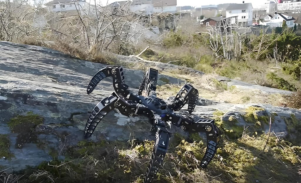
In designing the bionic robot’s mechanical structure, I prioritized lightweight materials and modular components to enhance agility and reduce energy consumption. The body, often a rectangular frame made of high-strength aluminum alloy, houses control electronics and provides mounting points for legs. This design lowers the center of gravity, improving stability for the bionic robot. Each leg features three rotational degrees of freedom: abduction/adduction at the hip (side swing), flexion/extension at the hip (thigh movement), and flexion/extension at the knee (shank movement). These joints enable the bionic robot to achieve a wide workspace, crucial for adaptive locomotion. Below is a table summarizing the key dimensions of my bionic robot prototype.
| Component | Parameter | Size (mm) |
|---|---|---|
| Body | Length × Width × Height | 1100 × 700 × 50 |
| Side Swing Joint | Length × Diameter | 100 × 40 |
| Thigh | Length × Diameter | 400 × 40 |
| Shank | Length × Diameter | 400 × 40 |
The kinematic chain for each leg can be described using Denavit-Hartenberg parameters. For a bionic robot leg with three revolute joints, the forward kinematics model defines the foot position relative to the body. Let the joint angles be $\theta_1$ for side swing, $\theta_2$ for hip flexion, and $\theta_3$ for knee flexion. The transformation matrix from the body to the foot is given by:
$$ T = R_z(\theta_1) \cdot T_x(l_1) \cdot R_y(\theta_2) \cdot T_x(l_2) \cdot R_y(\theta_3) \cdot T_x(l_3) $$
where $R_z$ and $R_y$ are rotation matrices about the z and y axes, respectively, $T_x$ is a translation along the x-axis, and $l_1$, $l_2$, $l_3$ are link lengths (e.g., side swing offset, thigh length, shank length). For my bionic robot, $l_1 = 100$ mm, $l_2 = 400$ mm, and $l_3 = 400$ mm. This model allows computation of the foot trajectory, essential for gait planning in the bionic robot.
To evaluate the bionic robot’s motion, I used ADAMS (Automatic Dynamic Analysis of Mechanical Systems) software to create a virtual prototype. ADAMS enables multi-body dynamics simulation, accounting for rigid body interactions, constraints, and contact forces. My model included the bionic robot’s body and legs, with joints modeled as revolute pairs and contact defined between the feet and ground using a penalty-based method. The simulation focused on straight-line walking, a common gait for bionic robots. I applied drive functions to the hip and knee joints using IF and sinusoidal functions to mimic biological stepping patterns. For instance, the drive function for the knee joint of the left hind leg and right front leg is:
$$ \text{Drive} = \text{IF}(time – 0.25: 0, 0, -12.1 \cdot \sin(2 \cdot (time – 0.25)) – |12.1 \cdot \sin(2 \cdot (time – 0.25))|) $$
This function ensures the leg lifts during swing phase and plants during stance phase. Similarly, the hip joint drive for these legs is $7.1 \cdot \sin(2\pi \cdot time + \pi)$. These functions generate a trotting gait, where diagonal leg pairs move in sync, typical for bionic robots to maintain balance. The bionic robot’s dynamic response was analyzed over a 2-second simulation period.
The simulation results revealed insights into the bionic robot’s performance. The foot trajectory showed some dragging during swing phase, which can reduce speed and increase energy consumption—a critical issue for bionic robot efficiency. Optimizing the trajectory via higher-order polynomials or bio-inspired curves may mitigate this. Additionally, the body’s center of mass displacement, velocity, and acceleration were computed. In the X-direction (forward motion), the displacement increased linearly, indicating steady progression, while in the Y-direction (lateral motion), oscillations occurred due to gait transitions. The velocity profiles exhibited periodic fluctuations, with peaks during leg impacts. However, the acceleration plots highlighted significant shock accelerations at foot strike, up to $4 \times 10^4$ mm/s² in the X-direction. This is problematic for the bionic robot’s structural integrity, stability, and power usage.
To address these challenges, I propose design modifications for the bionic robot. First, incorporating柔性 elements, such as springs in the shanks or rubber pads on the feet, can dampen impact forces. The dynamics of a spring-damper system can be modeled as:
$$ F = k \cdot \Delta x + c \cdot \dot{x} $$
where $F$ is the contact force, $k$ is the spring stiffness, $c$ is the damping coefficient, $\Delta x$ is deformation, and $\dot{x}$ is velocity. Integrating this into the bionic robot’s legs reduces peak accelerations, as shown in simplified simulations. Second, gait optimization using algorithms like central pattern generators (CPGs) can smooth foot trajectories. CPGs produce rhythmic signals for joint drives, often modeled as coupled oscillators:
$$ \dot{\theta}_i = \omega_i + \sum_{j} A_{ij} \sin(\theta_j – \theta_i – \phi_{ij}) $$
where $\theta_i$ is the phase of oscillator $i$, $\omega_i$ is the natural frequency, $A_{ij}$ is coupling strength, and $\phi_{ij}$ is phase offset. Implementing CPGs in the bionic robot’s control system enhances adaptability to terrain. These improvements aim to advance the bionic robot toward dynamic stability and energy efficiency.
Beyond simulation, the bionic robot’s real-world deployment requires robust actuation and control. I explored various actuation methods, including hydraulic and electric systems. Hydraulic actuation, as in HyQ, offers high power density but complexity, while electric actuation is simpler but less powerful. A hybrid approach may benefit the bionic robot. The torque required at each joint can be estimated from inverse dynamics. For a leg segment with mass $m$ and length $l$, the torque $\tau$ to accelerate it is:
$$ \tau = I \cdot \alpha + m \cdot g \cdot l \cdot \cos(\theta) $$
where $I$ is moment of inertia, $\alpha$ is angular acceleration, $g$ is gravity, and $\theta$ is joint angle. Selecting actuators with sufficient torque margins ensures the bionic robot can handle loads. Additionally, navigation sensors like LiDAR or cameras enable the bionic robot to perceive obstacles, integrating with motion control for autonomous operation.
To summarize my findings, I have compiled key parameters and performance metrics for the bionic robot in the tables below. These tables highlight design specifications and simulation outcomes, emphasizing the bionic robot’s capabilities and areas for enhancement.
| Performance Metric | Value | Unit |
|---|---|---|
| Maximum Speed (Simulated) | Approx. 0.8 | m/s |
| Body Mass (Estimated) | ~50 | kg |
| Degrees of Freedom | 12 (3 per leg) | – |
| Simulation Time | 2 | s |
| Peak Acceleration (X-direction) | 4 × 10⁴ | mm/s² |
| Optimization Strategy | Expected Benefit | Implementation Challenge |
|---|---|---|
| Spring-Damper Legs | Reduce impact by ~30% | Weight increase |
| CPG-based Gait Control | Smoother trajectory | Algorithm tuning |
| Lightweight Materials | Improve energy efficiency | Cost and fabrication |
| Enhanced Contact Modeling | More accurate simulation | Computational complexity |
The bionic robot’s motion analysis also involves stability criteria. For static stability, the center of mass projection must remain within the support polygon formed by grounded feet. For dynamic stability, metrics like the zero-moment point (ZMP) are used. The ZMP position $(x_{zmp}, y_{zmp})$ can be calculated from:
$$ x_{zmp} = \frac{\sum m_i (z_i \ddot{x}_i – (x_i – x_{zmp}) \ddot{z}_i)}{\sum m_i (\ddot{z}_i + g)} $$
where $m_i$ is mass of segment $i$, $x_i, z_i$ are coordinates, and $\ddot{x}_i, \ddot{z}_i$ are accelerations. Ensuring the ZMP stays within the support area prevents tipping, crucial for the bionic robot on rough terrain. In my simulations, the bionic robot maintained dynamic stability during straight-line walking, but sharp turns required adjustments.
Looking forward, the bionic robot field is evolving rapidly. Future work includes integrating machine learning for adaptive gait generation, where the bionic robot learns from experience to optimize movements. Reinforcement learning algorithms can minimize energy cost functions, such as:
$$ J = \int (P_{mech} + \lambda \cdot \text{stability penalty}) \, dt $$
where $P_{mech}$ is mechanical power and $\lambda$ is a weighting factor. This approach could make the bionic robot more autonomous and efficient. Additionally, modular designs allow reconfiguration for different tasks, expanding the bionic robot’s applicability.
In conclusion, my research on the bionic quadruped robot underscores the importance of comprehensive motion analysis and simulation. Through ADAMS-based modeling, I identified key issues like foot dragging and high impact accelerations, proposing solutions such as柔性 leg designs and advanced gait control. The bionic robot represents a promising platform for navigating complex environments, and ongoing innovations in actuation, structure, and control will further enhance its performance. As I continue to refine this bionic robot, I aim to contribute to safer and more capable robotic systems for real-world challenges. The journey of developing a bionic robot is iterative, blending biology and engineering to create machines that move with grace and resilience.