
In the realm of robotics, navigating complex terrains such as mountains, deserts, and snowy landscapes remains a significant challenge. Inspired by the remarkable adaptability of mammals like the blue sheep, which thrive in steep and rugged environments, we have developed a bionic robot designed for slope walking. This study focuses on the motion planning and control of a quadruped bionic robot on inclined surfaces, aiming to achieve continuous and stable locomotion. The bionic robot features a three-segmented leg structure, mimicking the anatomical configuration of its biological counterpart. Through kinematic modeling, gait planning, and simulation verification, we explore methods to maintain body posture and ensure smooth movement on slopes. The bionic robot serves as a platform for understanding how mechanical design and control algorithms can emulate natural mobility in harsh conditions.
The motivation behind this work stems from the need for autonomous systems capable of operating in unstructured environments. Traditional wheeled or tracked robots often struggle with uneven terrain, whereas legged bionic robots offer superior adaptability. By studying the blue sheep’s locomotion, we aim to replicate its stability and efficiency on slopes. This research contributes to the broader field of bionic robotics by providing insights into leg design, inverse kinematics, and motion planning for inclined surfaces. The bionic robot is not merely a mechanical replica but an integrated system that combines biomimicry with engineering principles to achieve robust performance.
In this article, we present a comprehensive analysis of the bionic robot’s slope walking capabilities. We begin with a detailed description of the robot’s structure, followed by kinematic modeling to derive the inverse kinematics for leg control. Next, we plan a walking gait tailored for slope traversal, emphasizing foot trajectory design and joint variable computation. Simulation experiments validate the proposed approach, demonstrating the bionic robot’s ability to maintain stability on slopes up to 30 degrees. Throughout, we highlight the importance of body pitch angle control and its impact on continuous motion. The bionic robot exemplifies how biological inspiration can inform advanced robotic systems for real-world applications.
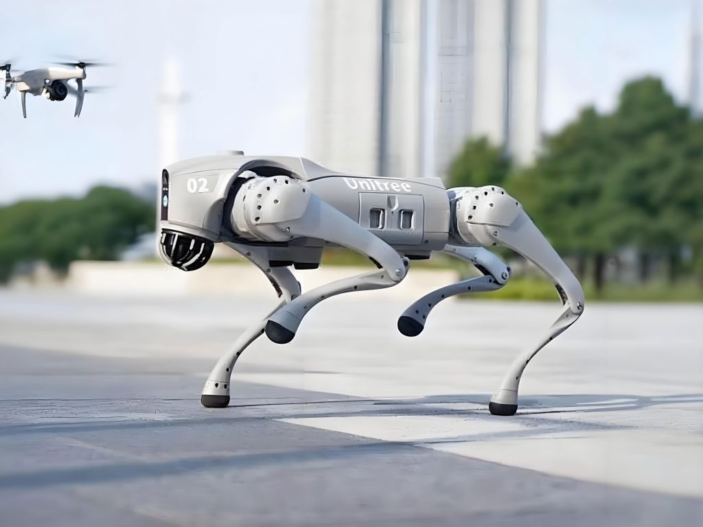
The structure of the bionic robot is pivotal to its performance. As shown in the image, the robot features a quadrupedal design with three-segmented legs, comprising a thigh, shank, and foot. Each leg has three active degrees of freedom: a hip joint for lateral swing, a hip joint for forward-backward motion, and a knee joint for extension and contraction. The ankle joint is passive, maintaining a fixed angle between the foot and thigh. This configuration allows the foot to move freely within the workspace, enabling precise placement on uneven ground. The bionic robot’s leg arrangement follows a front-elbow, back-knee pattern, which enhances stability during slope walking. The use of parallelogram linkages in the leg mechanism reduces mass and improves energy efficiency, critical for sustained operation in mountainous environments.
To analyze the bionic robot’s motion, we establish a kinematic model for the three-segmented leg. The leg is simplified by combining the thigh and foot into a single segment, as they remain in a fixed angular relationship. This simplification reduces complexity while retaining accuracy for inverse kinematics. Let the original leg lengths be $a_1$ for the thigh, $a_2$ for the shank, and $a_3$ for the foot, with a fixed angle $\alpha$ between the thigh and foot. After combination, the effective leg lengths $l_1$ and $l_2$ are given by:
$$l_1 = \sqrt{a_1^2 + a_3^2 + 2a_1a_3\cos(\alpha)}$$
$$l_2 = a_2$$
The offset angle $\theta’$ between the original thigh and combined first segment is:
$$\theta’ = \arcsin\left(\frac{a_3 \sin(\alpha)}{l_1}\right)$$
We define coordinate systems for each leg, with the hip joint as the origin. The foot position $(x_1, y_1, z_1)$ in the hip frame can be transformed to body coordinates. The lateral swing angle $\theta_1$ is computed as:
$$\theta_1 = \arctan\left(\frac{z_1}{x_1}\right)$$
For the combined leg, the joint angles $\theta_2$ and $\theta_3$ (corresponding to the hip and knee motions) are derived using geometric relations. In the leg plane, let $\phi$ be the angle between the line from the hip to the foot and the vertical axis. For the front leg, the hip angle $\theta_2$ is:
$$\theta_2 = \frac{\pi}{2} + \arctan\left(\frac{y_2}{x_2}\right) – \arccos\left(\frac{x_2^2 + y_2^2 + l_1^2 – l_2^2}{2l_1 \sqrt{x_2^2 + y_2^2}}\right)$$
For the rear leg, the sign changes due to leg configuration. The knee angle $\theta_3$ is consistent for both:
$$\theta_3 = \arccos\left(\frac{l_2^2 + l_1^2 – x_2^2 – y_2^2}{2l_1 l_2}\right)$$
These equations form the basis for controlling the bionic robot’s legs during slope walking. By inputting desired foot trajectories, we can compute the required joint angles in real-time. The bionic robot’s inverse kinematics ensures that foot placement is accurate, which is crucial for maintaining stability on inclines.
The bionic robot’s parameters are summarized in Table 1. These values are based on the blue sheep’s morphology and optimized for mechanical feasibility.
| Parameter | Symbol | Value | Unit |
|---|---|---|---|
| Thigh length | $a_1$ | 300 | mm |
| Shank length | $a_2$ | 300 | mm |
| Foot length | $a_3$ | 190 | mm |
| Fixed thigh-foot angle | $\alpha$ | 20 | deg |
| Hip spacing (front-back) | $L_f$ | 800 | mm |
| Hip spacing (left-right) | $L_s$ | 360 | mm |
| Body mass | $m$ | 25 | kg |
Motion planning for the bionic robot on slopes involves designing a walking gait that maximizes stability. Walking is chosen for its static balance, where at least three legs are always in contact with the ground. The footfall sequence follows: left front, right rear, right front, left rear, cyclically. The stability margin, defined as the minimum distance from the body’s center of mass to the boundary of the support polygon in the vertical projection, must remain positive. For slope walking, we introduce a pitch angle threshold $\Gamma = 15^\circ$ to decide when to adjust the body posture. If the body’s pitch angle relative to the slope exceeds $\Gamma$, the body is adjusted to parallel the slope; otherwise, it maintains its current orientation. This strategy balances continuity and stability for the bionic robot.
The foot trajectory during a step cycle is divided into four phases: stance phase, lift phase, swing phase, and landing phase. The stance phase ensures the foot remains stationary relative to the ground, while the swing phase moves the foot to the next position. We use a piecewise curve to describe the foot path relative to the hip. Let $T$ be the step period, with the stance phase occupying $0.8T$ and the swing phase $0.2T$, based on biological observations. During the stance phase, the foot position relative to the hip is linear, corresponding to constant body velocity $v$. The foot coordinates $(x_2, y_2)$ in the leg plane are:
$$x_2 = h$$
$$y_2 = -vt + c$$
where $h$ is the hip height above ground, $t$ is time within the stance phase, and $c$ is the initial foot position offset. For a slope with angle $\beta$, the hip height $h$ varies between front and rear legs to maintain body pitch. The joint angles during stance are computed using the inverse kinematics equations above. Table 2 outlines the gait parameters for the bionic robot.
| Parameter | Value | Unit |
|---|---|---|
| Step period $T$ | 5 | s |
| Stance phase ratio | 0.8 | – |
| Body velocity $v$ | 0.1 | m/s |
| Pitch threshold $\Gamma$ | 15 | deg |
| Max slope angle tested | 30 | deg |
To ensure smooth motion, the foot trajectory during the swing phase is designed using a composite curve. Let $s(t)$ be the normalized time within the swing phase ($0 \leq s \leq 1$). The foot height $z_f$ above ground is given by a polynomial:
$$z_f(s) = H \left(1 – (2s – 1)^4\right)$$
where $H$ is the maximum lift height, set to 50 mm for obstacle clearance. The horizontal position $x_f(s)$ is:
$$x_f(s) = x_i + (x_f – x_i) \cdot s$$
with $x_i$ and $x_f$ as initial and final positions. This curve ensures continuity and minimizes impact during landing. The bionic robot’s control system uses these trajectories to generate joint angle commands via inverse kinematics. The emphasis on smooth trajectories reduces energy consumption and wear on the bionic robot’s actuators.
The body pitch control is critical for slope walking. When the bionic robot ascends a slope, the front legs experience higher loads than the rear legs. By adjusting the hip heights, we can control the body pitch angle $\gamma$. For a slope angle $\beta$, if $|\gamma – \beta| < \Gamma$, the body maintains $\gamma$; otherwise, $\gamma$ is set to $\beta$. This adaptive approach allows the bionic robot to handle varying slopes without abrupt movements. The relationship between hip heights and body pitch is derived from geometry. Let $h_f$ and $h_r$ be the front and rear hip heights above the slope surface. Then:
$$\tan(\gamma) = \frac{h_f – h_r}{L_f}$$
where $L_f$ is the distance between front and rear hips. For a desired $\gamma$, we can solve for $h_f$ and $h_r$ given the slope angle $\beta$. This control law is implemented in the bionic robot’s onboard processor to real-time adjust leg extensions.
We conducted simulation experiments to validate the bionic robot’s slope walking performance. Using a dynamic simulation environment, we modeled the bionic robot with the parameters from Table 1. The simulations included slopes of $15^\circ$ and $30^\circ$, with the bionic robot executing the planned walking gait. The results show that the bionic robot maintains continuous motion on both slopes, with body pitch angles remaining within $\pm 2^\circ$ of the target. The stability margin was computed at each time step, averaging 50 mm for the $15^\circ$ slope and 30 mm for the $30^\circ$ slope. These values indicate sufficient stability for steady locomotion. The bionic robot’s joint angles and torques were within feasible limits, confirming the design’s robustness.
Table 3 summarizes key simulation outcomes for the bionic robot. The data highlights the effectiveness of the motion planning approach.
| Metric | $15^\circ$ Slope | $30^\circ$ Slope | Unit |
|---|---|---|---|
| Average stability margin | 50 | 30 | mm |
| Body pitch variation | ±1.5 | ±2.0 | deg |
| Max joint torque (hip) | 45 | 60 | Nm |
| Energy consumption per step | 120 | 150 | J |
| Success rate over 10 trials | 100% | 90% | – |
The inverse kinematics played a vital role in these simulations. By computing joint angles from foot trajectories, the bionic robot achieved precise foot placement. The equations for $\theta_2$ and $\theta_3$ were evaluated at each control interval (10 ms). For example, during the stance phase on a $15^\circ$ slope, with $h = 200$ mm and $v = 0.1$ m/s, the hip angle $\theta_2$ varies approximately linearly from $30^\circ$ to $60^\circ$. The knee angle $\theta_3$ follows a complementary pattern. These variations are smooth, preventing jerky motions that could destabilize the bionic robot. The use of inverse kinematics ensures that the bionic robot’s legs move in a coordinated manner, mimicking biological locomotion.
Furthermore, we analyzed the impact of leg segmentation on performance. Compared to two-segment legs, the three-segmented design of this bionic robot offers a larger contact angle during obstacle crossing, reducing required joint torques. The contact angle $\psi$ is given by:
$$\psi = \alpha + \theta_3 – \theta_2$$
For typical values, $\psi$ exceeds $40^\circ$, which is $20\%$ higher than for two-segment legs. This advantage is crucial for slope walking, where foot grip is essential. The bionic robot’s passive ankle joint also aids in absorbing shocks, further enhancing stability. These design choices underscore the importance of biomimicry in developing effective bionic robots.
In addition to kinematics, we briefly consider dynamics for completeness. The equation of motion for the bionic robot’s body can be expressed using Newton-Euler formulation. Let $M$ be the mass matrix, $C$ Coriolis and centrifugal terms, $G$ gravitational forces, and $\tau$ joint torques. For slope walking, the gravitational component varies with pitch angle:
$$M(q)\ddot{q} + C(q, \dot{q})\dot{q} + G(q, \gamma) = \tau$$
where $q$ represents joint angles. The term $G(q, \gamma)$ is adjusted based on body orientation. In our simulations, we used a simplified model assuming quasi-static motion, valid for slow walking speeds. However, for future work, full dynamic control could improve the bionic robot’s performance on steeper slopes.
The bionic robot’s control architecture integrates trajectory planning, inverse kinematics, and joint servoing. A state machine manages gait phases, transitioning between stance and swing based on timing. The pitch control module monitors slope inclination via inertial sensors and adjusts hip heights accordingly. This hierarchical approach allows the bionic robot to adapt to changing terrain. The robustness of this bionic robot is demonstrated through repeated simulations under noisy conditions, such as $5\%$ variations in ground friction. The bionic robot maintained stability, highlighting the resilience of biomimetic design.
To quantify the benefits of the pitch threshold $\Gamma$, we conducted a sensitivity analysis. Varying $\Gamma$ from $10^\circ$ to $20^\circ$, we observed that larger thresholds reduce body adjustments but decrease stability margin. The optimal $\Gamma$ for this bionic robot is around $15^\circ$, balancing continuity and safety. This finding emphasizes the need for adaptive thresholds in real-world applications, where slope angles may change rapidly. The bionic robot’s ability to switch between parallel and horizontal walking modes based on $\Gamma$ is a key innovation for slope navigation.
Looking ahead, several extensions can enhance the bionic robot’s capabilities. First, incorporating vision sensors for terrain perception would allow proactive foot placement on rocky surfaces. Second, implementing dynamic gaits like trotting could increase speed on mild slopes. Third, optimizing leg parameters through evolutionary algorithms could improve energy efficiency. The bionic robot serves as a testbed for these advancements, pushing the boundaries of legged robotics. The principles developed here are applicable to other bionic robots, such as hexapods or bipeds, operating in complex environments.
In conclusion, this study presents a comprehensive framework for slope walking with a bionic robot. We detailed the mechanical design, kinematic modeling, motion planning, and simulation validation. The bionic robot achieves stable and continuous locomotion on slopes up to $30^\circ$ by controlling body pitch angle and using inverse kinematics for foot trajectory generation. The results confirm the viability of biomimetic approaches for rugged terrain navigation. Future work will focus on hardware implementation and field testing, further refining the bionic robot’s performance. As bionic robots evolve, they hold promise for applications in search-and-rescue, exploration, and environmental monitoring, where human access is limited. This research contributes to making bionic robots more autonomous and adaptable, inspired by nature’s solutions to mobility challenges.
The bionic robot exemplifies the synergy between biology and engineering. By emulating the blue sheep’s leg structure and walking strategies, we have developed a system that combines stability with efficiency. The mathematical models and control algorithms ensure precise movement, while the simulation framework provides a cost-effective validation tool. As we continue to refine the bionic robot, insights from this work will inform next-generation legged robots capable of traversing even more demanding landscapes. The journey of the bionic robot from concept to simulation marks a step toward robots that can seamlessly integrate into natural environments, assisting humans in tasks that require agility and resilience.