
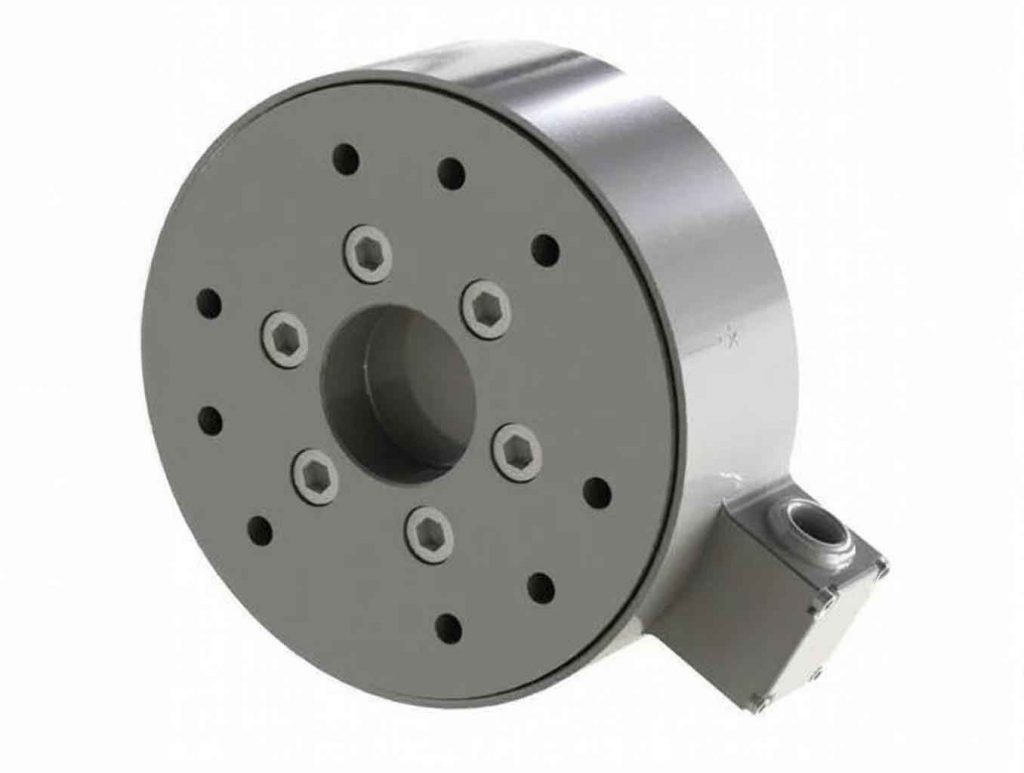
In modern industrial and robotic applications, the accurate measurement of multi-dimensional forces is critical for tasks requiring precision and reliability. The six-axis force sensor plays a pivotal role in capturing forces and moments along three translational and three rotational axes. However, dynamic loading environments often introduce significant noise pollution, severely degrading the measurement accuracy of these sensors. Traditional filtering methods, such as the extended Kalman filter (EKF), struggle to achieve optimal performance due to difficulties in accurately estimating the system noise matrix. To address these challenges, we propose a novel chaotic invasive weed optimization-based extended Kalman filter (CIWO-EKF) algorithm. This approach leverages the chaotic properties of invasive weed optimization to refine the system noise matrix, thereby enhancing the filtering performance for six-axis force sensors. By integrating global and local search mechanisms, our method ensures robust and real-time noise suppression, making it highly suitable for dynamic applications.
The six-axis force sensor typically employs a resistive strain gauge configuration, where deformations in elastic elements under load produce electrical signals via Wheatstone bridges. In dynamic scenarios, factors such as thermal noise from strain gauges, amplifier circuits, and electromagnetic interference introduce colored noise, complicating signal processing. The EKF, a nonlinear state estimation technique, is widely used for such applications but relies heavily on the accuracy of the system noise covariance matrix. Inaccurate noise matrices can lead to increased uncertainty and suboptimal filtering. Previous optimization attempts, including genetic algorithms (GA) and particle swarm optimization (PSO), have shown limitations in convergence speed and local optima avoidance. Our CIWO-EKF algorithm overcomes these issues by combining the invasive weed optimization (IWO) with chaotic sequences, enabling efficient global exploration and precise local refinement.
To model the six-axis force sensor, we focus on the lower E-membrane structure, which detects tangential forces (FX, FY) and the normal force (FZ). The membrane’s response to sinusoidal excitation forces is derived from modal superposition theory. Under zero initial conditions, the dynamic deflection of the lower E-membrane can be expressed as an infinite series of mode shapes and time functions. For practical implementation, we consider the first six dominant modes to balance computational efficiency and accuracy. The relationship between deflection and strain is key to constructing the nonlinear state-space model. The radial strain ε(r, φ, t) at the strain gauge locations is derived from the deflection w(r, φ, t), leading to a discrete-time system representation. The state equation incorporates terms for strain evolution, control inputs, and noise effects, while the measurement equation accounts for observed signals corrupted by Gaussian noise.
The state-space model for the six-axis force sensor’s lower E-membrane is formulated as follows. Let Xk be the state vector at time k, comprising strain and mode-related variables. The nonlinear discrete-time state equation is:
$$ \epsilon(k+1) = \epsilon(k) + 2T w \sin(w k) \sum_{j=1}^{N} N_j \sum_{j=1}^{N} \frac{N_j \sin(\omega_j k)}{\omega_j} + T w N_j \sum_{j=1}^{N} (\cos(w k) – \cos(\omega_j k)) + T A \epsilon^2(k) – T \left( \sum_{j=1}^{N} N_j \right)^2 \sin^2(w k) $$
where T is the sampling period, w is the excitation frequency, ωj are the natural frequencies, Nj are strain gauge coefficients, and A is a noise-related constant. The coefficients Nj are defined as:
$$ N_j = -\frac{h}{2m} \frac{\partial^2 W_m(r, \phi)}{\partial r^2} \frac{K_j}{\omega_j^2 – w^2} $$
Here, h is the membrane thickness, m is the mass per unit area, and Wm(r, φ) is the mode shape function. To handle colored noise, we apply a Gaussian-Markov model for whitening, resulting in an augmented state-space model for EKF:
$$ X_{k+1} = \Phi_{k+1,k} X_k + G_{k+1,k} U_k + \Gamma_{k+1,k} \eta_k $$
$$ Z_{k+1} = H X_{k+1} + V_{k+1} $$
The state vector Xk+1 includes strain and mode amplitudes, Uk is the control input vector, ηk is white noise, and Vk+1 is measurement noise with covariance Rσ. The matrices Φ, G, and Γ are derived from linearization and noise modeling. The system noise covariance matrix Qn is diagonal, with elements depending on the mode shapes and excitation parameters. Accurate estimation of Qn is crucial for EKF performance, as deviations can lead to filter divergence.
The standard EKF involves prediction and update steps. In the prediction step, the state and error covariance are projected forward:
$$ \hat{X}_{k+1|k} = \Phi_{k+1,k} \hat{X}_k + G_{k+1,k} U_k $$
$$ P_{k+1|k} = \Phi_{k+1,k} P_k \Phi_{k+1,k}^T + \Gamma_{k+1,k} Q_n \Gamma_{k+1,k}^T $$
The update step incorporates new measurements to refine the estimates:
$$ \hat{R}_{k+1} = (1 – d_{k+1}) \hat{R}_k + d_{k+1} \left[ (Z_{k+1} – H \hat{X}_{k+1|k}) (Z_{k+1} – H \hat{X}_{k+1|k})^T – H P_{k+1|k} H^T \right] $$
$$ K_{k+1} = P_{k+1|k} H^T (H P_{k+1|k} H^T + R_{k+1})^{-1} $$
$$ \hat{X}_{k+1} = \hat{X}_{k+1|k} + K_{k+1} (Z_{k+1} – H \hat{X}_{k+1|k}) $$
$$ P_{k+1} = (I – K_{k+1} H) P_{k+1|k} $$
Here, Kk+1 is the Kalman gain, and dk+1 is a forgetting factor. The measurement noise covariance R is estimated online, but Qn requires offline optimization. Our CIWO-EKF algorithm optimizes Qn by treating it as a diagonal matrix with six elements corresponding to the first six mode shapes. The optimization aims to minimize the mean squared error between the actual sinusoidal input and the filtered output.
The invasive weed optimization (IWO) algorithm mimics the colonization behavior of weeds. It starts with an initial population of solutions (weeds), which reproduce based on fitness. The number of seeds produced by each weed is:
$$ s = \frac{f – f_{\text{min}}}{f_{\text{max}} – f_{\text{min}}} (s_{\text{max}} – s_{\text{min}}) + s_{\text{min}} $$
where f is the fitness value, and smax and smin are the maximum and minimum seed counts. Seeds are dispersed in the search space with a standard deviation that decreases over iterations:
$$ \sigma_{\text{cur}} = \left( \frac{I_{\text{max}} – I}{I_{\text{max}}} \right)^u (\sigma_{\text{init}} – \sigma_{\text{final}}) + \sigma_{\text{final}} $$
where I is the current iteration, Imax is the maximum iterations, and u is a nonlinear modulation factor. To enhance local search, we integrate chaotic sequences using the Logistic map:
$$ y_{m+1} = \mu y_m (1 – y_m) $$
where μ is a control parameter, and m is the iteration index. Chaotic variables are mapped to the solution space to generate new candidates, improving exploration and avoiding local optima.
In CIWO-EKF, the fitness function for optimizing Qn is defined as the mean squared error between the reference sinusoidal signal and the EKF output:
$$ F_i = \frac{1}{N} \sum_{k=1}^{N} (K \sin(w k) – f(\hat{X}^i_k))^2 $$
where f(·) represents the filtered signal. The initial population for IWO is generated by Gaussian sampling around the first six mode shapes. After each IWO iteration, chaotic local search is applied to individuals with above-average fitness, guiding the population toward the global optimum. This hybrid approach ensures rapid convergence and high accuracy.
For experimental validation, we consider a six-axis force sensor with a lower E-membrane of specific dimensions: inner radius 50 mm, outer radius 100 mm, and thickness 2 mm. Strain gauges are positioned at strategic points, and parameters such as excitation frequency and amplitude are set to simulate dynamic conditions. The system matrices are derived based on the first six natural frequencies and mode shapes. We compare CIWO-EKF with GA-EKF and PSO-EKF in terms of filtering accuracy, convergence speed, and robustness to disturbances.
The table below summarizes the parameters used in the optimization algorithms:
| Parameter | Value |
|---|---|
| Initial Population Size | 20 |
| Maximum Iterations | 50 |
| Initial Standard Deviation | 2.5 |
| Final Standard Deviation | 0.01 |
| Seed Range [smin, smax] | [0, 5] |
| Nonlinear Factor u | 3 |
In the case of fixed amplitude and frequency excitation, the CIWO-EKF demonstrates superior filtering performance. The following table compares the mean squared errors (MSE) for different algorithms under various conditions:
| Algorithm | MSE (No Disturbance) | MSE (Frequency Disturbance) | MSE (Amplitude Disturbance) |
|---|---|---|---|
| GA-EKF | 1.9504 × 10⁻³ | 2.2356 × 10⁻³ | 2.3131 × 10⁻³ |
| PSO-EKF | 1.1615 × 10⁻³ | 1.2969 × 10⁻³ | 1.3456 × 10⁻³ |
| CIWO-EKF | 0.76979 × 10⁻³ | 0.93092 × 10⁻³ | 0.94835 × 10⁻³ |
The results indicate that CIWO-EKF reduces MSE by approximately 60.53% compared to GA-EKF and 33.72% compared to PSO-EKF in undisturbed cases. Under disturbances, such as sudden changes in excitation frequency or amplitude, CIWO-EKF maintains stability and quickly converges to the true state, showcasing its robustness. The convergence curves of the fitness function further highlight the efficiency of CIWO, with faster descent and lower final values than other methods.
To evaluate computational complexity, we measure the execution time for each algorithm to achieve similar MSE levels. The table below presents the average runtimes for 50 sampling points:
| Algorithm | Runtime (No Disturbance) | Runtime (Frequency Disturbance) | Runtime (Amplitude Disturbance) |
|---|---|---|---|
| Standard EKF | 0.5263 s | 0.6538 s | 0.6429 s |
| GA-EKF | 0.6172 s | 0.7326 s | 0.7292 s |
| PSO-EKF | 0.5939 s | 0.7148 s | 0.6935 s |
| CIWO-EKF | 0.5583 s | 0.6823 s | 0.6647 s |
CIWO-EKF offers a favorable balance between accuracy and computational cost, with runtimes close to standard EKF but significantly improved performance. This makes it practical for real-time applications in six-axis force sensors. The algorithm’s ability to handle dynamic coupling effects in multi-directional loading scenarios, though not fully explored here, suggests potential for future research in comprehensive decoupling strategies.
In conclusion, the CIWO-EKF algorithm effectively addresses the challenges of noise pollution and system noise matrix estimation in six-axis force sensors. By combining the global search capabilities of invasive weed optimization with the local refinement of chaotic sequences, it achieves high filtering accuracy, robustness, and real-time performance. Experimental results validate its superiority over traditional optimization methods, paving the way for enhanced sensor applications in dynamic environments. Future work will focus on extending this approach to multi-directional force measurements and dynamic decoupling techniques for full six-axis utilization.