
Humanoid robots have emerged as one of the most promising fields in modern robotics, aiming to combine the efficiency and reliability of machines with the flexibility and adaptability of human morphology. In my research, I focus on the design and control of a hydraulic actuator intended for humanoid robot joints, with special emphasis on compliant control. The core objective is to enable humanoid robots to interact safely and naturally with unknown environments, especially when physical contact is unavoidable. Traditional rigid actuators often fail to provide the required adaptability for human-robot interaction, and thus I propose the use of an electro-hydrostatic actuator (EHA) as a compact, high-power-density joint actuator. This work covers the complete development process, including mechanical design, nonlinear mathematical modeling, high-precision position control, compliance control, and experimental validation.
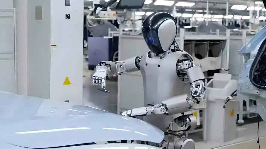
The rapid advancement of humanoid robots has led to increasing demands on joint actuators. These actuators must provide high torque, fast response, accurate position tracking, and, most importantly, compliance to ensure safe interactions. In this thesis, I investigate the compliant control problem for a hydraulic joint actuator based on EHA technology. The EHA integrates an electric motor, a bidirectional pump, and a symmetric cylinder into one compact unit, eliminating the need for bulky centralized hydraulic power supplies. This design philosophy aligns perfectly with the concept of structural and functional integration for humanoid robots, where every component must serve both structural and actuation purposes. The main contributions of my research are the detailed nonlinear model of the EHA, the design of advanced position controllers, and the development of an adaptive compliance control strategy that effectively reduces steady-state force errors during contact tasks.
Design of the Joint Hydraulic Actuator for Humanoid Robots
Humanoid robots operate under two distinct types of working conditions: continuous contact tasks and intermittent contact tasks. In continuous contact tasks, such as polishing or grinding, the actuator must maintain a stable contact force while following a desired trajectory. In intermittent contact tasks, such as walking, the leg repeatedly contacts and separates from the ground, producing periodic impact forces. Both scenarios require the actuator to exhibit compliant behavior, meaning that the output force should be regulated dynamically in response to position deviations. To meet these requirements, I designed an EHA-based joint actuator that can be embedded into the structural framework of a humanoid robot.
The EHA system schematic is shown below in the form of a hydraulic circuit. The system consists of a servo motor driving a fixed-displacement bidirectional piston pump, two relief valves for pressure protection, two check valves for oil replenishment, a spring-loaded accumulator tank, a symmetric hydraulic cylinder, and a group of balancing valves. The displacement sensor provides feedback for closed-loop position control, while pressure sensors monitor the chamber pressures. The use of a symmetric cylinder simplifies the pressure-flow relationship and allows the same dynamic performance in both directions. The motor speed and direction directly control the pump flow rate, and therefore the cylinder velocity. This pump-controlled architecture avoids throttling losses and provides higher energy efficiency compared with valve-controlled systems.
| Component | Parameter | Value |
|---|---|---|
| Symmetric cylinder | Bore diameter | 63 mm |
| Rod diameter | 35 mm | |
| Stroke | ±50 mm | |
| Maximum load | 20000 N | |
| Servo motor | Rated power | 400 W |
| Rated speed | 3000 r/min | |
| Piston pump | Displacement | 1 ml/r |
| Rated pressure | 30 MPa | |
| Weight | 0.45 kg |
The design process started with the specification of the maximum output force. For a humanoid robot knee joint, a torque of approximately 800 N·m is required when the moment arm is 0.04 m, which corresponds to a linear force of 20000 N. The hydraulic cylinder was selected with a bore of 63 mm and a rod of 35 mm, giving an effective piston area that can generate the required force at a working pressure of about 9.28 MPa. The cylinder wall thickness was calculated to be at least 6 mm based on the maximum pressure and material yield strength; I chose 13.5 mm to provide a sufficient safety margin. The maximum flow rate was determined from the required maximum speed of 20 mm/s, yielding a pump displacement of approximately 1 ml/r. The selected pump is an axial piston pump with seven pistons, rated at 1 ml/r and up to 4000 r/min. The servo motor was chosen to deliver 400 W at 3000 r/min, which is sufficient for the maximum power demand of 285 W.
Nonlinear Mathematical Modeling of the Joint Actuator
To achieve high-precision position control and robust compliance control, an accurate model of the EHA is essential. The system exhibits several nonlinearities that significantly affect control performance. I identified two dominant nonlinear factors: the efficiency variation of the piston pump and the nonlinear friction inside the hydraulic cylinder. While other effects such as flow pulsation and oil compressibility are present, their influence is secondary compared with these two. I therefore developed a detailed nonlinear model that captures the pump volumetric losses and the LuGre friction model for the cylinder.
Pump Nonlinear Model
The volumetric loss of the pump consists of leakage losses from the piston–cylinder interface, the slipper–swashplate interface, and the valve plate, plus the compression loss. The total volumetric loss can be expressed as the sum of the individual leakage flow rates:
$$Q_v = \sum Q_{Li} + Q_c$$
where $Q_{Li}$ represents the leakage from each friction pair and $Q_c$ is the oil compression loss. The piston pair leakage is given by:
$$Q_{L1} = \sum_{i=1}^{z} \frac{\pi d_p \delta_p^3 (1 + 1.5 \varepsilon^2) \Delta p_{pi}}{12 \mu L_i}$$
where $d_p$ is the piston diameter, $\delta_p$ is the radial clearance, $\Delta p_{pi}$ is the pressure difference, $\mu$ is the dynamic viscosity, $\varepsilon$ is the eccentricity, and $L_i$ is the contact length. The slipper pair leakage and valve plate leakage can be similarly expressed with geometric parameters. Consequently, the volumetric efficiency of the pump is defined as:
$$\eta_v = 1 – \frac{\sum Q_{Li} + Q_c}{Q_T}$$
where $Q_T = D_p n / 60$ is the theoretical flow. Taking the mechanical efficiency as $\eta_m = 0.92$, the total efficiency model is obtained as:
$$\eta = 0.92 – \frac{102.33(p_1 – p_2) + 0.09n}{1000 n}$$
This nonlinear efficiency model was incorporated into the simulation and control design.
Cylinder Nonlinear Model
For the hydraulic cylinder, the flow continuity equation can be written for the two chambers. Assuming no external leakage and a symmetric cylinder, the load flow equation is:
$$Q_L = A_p \dot{x}_p + C_i p_L + \frac{V_t}{4 \beta_e} \dot{p}_L$$
where $A_p$ is the piston effective area, $x_p$ is the piston displacement, $p_L$ is the load pressure, $C_i$ is the internal leakage coefficient, $V_t$ is the total trapped oil volume, and $\beta_e$ is the effective bulk modulus. The force balance equation for the piston is:
$$A_p p_L = M \ddot{x}_p + B_c \dot{x}_p + f_f + F_L$$
where $M$ is the total mass, $B_c$ is the viscous damping coefficient, $f_f$ is the nonlinear friction force, and $F_L$ is the external load. I used the LuGre friction model to represent the friction behavior:
$$
\begin{aligned}
\frac{dz}{dt} &= \dot{x}_p – \frac{\sigma_0 |\dot{x}_p|}{g(\dot{x}_p)} z \\
g(\dot{x}_p) &= f_c + (f_s – f_c) e^{-(\dot{x}_p/v_s)^2}
\end{aligned}
$$
where $z$ is the bristle deflection, $\sigma_0$ is the bristle stiffness, $\sigma_1$ is the bristle damping, $\sigma_2$ is the viscous friction coefficient, $f_c$ is the Coulomb friction, $f_s$ is the static friction, and $v_s$ is the Stribeck velocity. After fitting the model to experimental data, the friction force was approximated as:
$$f_f = 164.78 – \frac{165.66}{1 + (\dot{x}_p / 0.02)^{2.28}}$$
This nonlinear friction model captures the difference between static and kinetic friction, which is crucial for high-precision position tracking at low speeds.
High-Precision Position Control for Humanoid Robot Joints
The performance of compliant control strongly depends on the inner position loop. For humanoid robots, the joint actuator must track desired trajectories accurately and quickly. I implemented and compared four control strategies: PID control, sliding mode control (SMC), backstepping control, and adaptive backstepping control based on model parameter estimation. The simulation environment was constructed using AMESim for the hydraulic system and Simulink for the control algorithms. The two software platforms were coupled through a co-simulation interface, allowing the nonlinear hydraulic model to interact with the controller.
PID Control
The classic PID controller is widely used in industrial applications due to its simple structure. The control law is:
$$u(t) = K_p e(t) + K_i \int_0^t e(\tau) d\tau + K_d \frac{de(t)}{dt}$$
where $e(t) = x_d(t) – x(t)$ is the tracking error, $K_p$, $K_i$, and $K_d$ are the proportional, integral, and derivative gains. The PID controller serves as a baseline for comparison.
Sliding Mode Control
Sliding mode control is robust to parameter uncertainties and external disturbances. I defined the state variables as $[x_1, x_2, x_3]^T = [x_p, \dot{x}_p, \ddot{x}_p]^T$ and constructed the sliding surface as:
$$s = c_1 e_1 + c_2 e_2 + e_3$$
Using an exponential reaching law, the control input is:
$$u = u_{eq} + u_{sw}$$
where $u_{eq}$ is the equivalent control derived from $\dot{s}=0$, and $u_{sw}$ is the switching control:
$$u_{sw} = \frac{V_t M}{4 \beta_e A_p D_p \eta} \left( k_1 \operatorname{sgn}(s) + k_2 s \right)$$
The stability is guaranteed by the Lyapunov function $V = \frac{1}{2} s^2$, whose derivative is negative definite when $k_1>0$ and $k_2>0$.
Backstepping Control
Backstepping control is a recursive design methodology suitable for strict-feedback nonlinear systems. I defined the errors as $e_1 = x_1 – x_{1d}$, $e_2 = x_2 – \alpha_1$, $e_3 = x_3 – \alpha_2$, where $\alpha_1$ and $\alpha_2$ are virtual control signals. The control law was derived step by step to stabilize each subsystem. The final backstepping control input is:
$$u = \frac{V_t}{4 \beta_e A_p D_p \eta} \left[ \frac{A_p \beta_e}{V_t} x_3 + \frac{C_i \beta_e B_c}{V_t M} x_2 + \frac{C_i \beta_e}{V_t M} F_L + \ddot{x}_{1d} + (k_1 + k_2 + k_3) e_2 + (k_1 k_2 + k_2 k_3 + k_1 k_3) e_3 + k_1 k_2 k_3 \int e_1 dt \right]$$
In practice, I used a simplified form with carefully tuned gains to achieve a stable response.
Adaptive Backstepping Control
To handle parameter uncertainties, I enhanced the backstepping controller with an adaptive law that estimates the unknown model parameters online. The system model was rewritten as:
$$\dot{x}_3 = \theta_1 x_2 – \theta_2 x_3 + \theta_3 u + d$$
where $\theta_i$ represent uncertain parameters. The adaptive backstepping control law and parameter update laws are designed as:
$$u = \frac{1}{\hat{\theta}_3} \left[ \hat{\theta}_1 x_2 – \hat{\theta}_2 x_3 + \ddot{x}_{1d} – \hat{\theta}_1 x_2 – \hat{\theta}_2 x_3 + k_1 e_1 + k_2 e_2 + k_3 e_3 + \cdots \right]$$
$$\dot{\hat{\theta}}_1 = \alpha_1 e_3 x_2, \quad \dot{\hat{\theta}}_2 = \alpha_2 e_3 x_3, \quad \dot{\hat{\theta}}_3 = \alpha_3 e_3 u$$
The Lyapunov function including parameter errors ensures that the closed-loop system is asymptotically stable.
Simulation Results for Position Control
I performed co-simulations for a 30 mm step command and a sinusoidal command with amplitude 30 mm and period 20 s. The following performance indices were calculated:
- Mean absolute error (MAE): $E_{MAE} = \frac{1}{N}\sum_{i=1}^{N} |e(i)|$
- Root mean square error (RMSE): $E_{RMSE} = \sqrt{\frac{1}{N}\sum_{i=1}^{N} (e(i) – \bar{e})^2}$
- Integral of time-weighted absolute error (ITAE): $E_{ITAE} = \sum_{i=1}^{N} T_s |e(i)|$
The simulation results for the step response are summarized in the following table.
| Controller | Rise time (s) | MAE (mm) | RMSE (mm) | ITAE (mm·s) |
|---|---|---|---|---|
| PID | 2.51 | 0.002181 | 0.061438 | 1.020650 |
| Sliding mode | 1.65 | 0.002162 | 0.061154 | 1.004391 |
| Backstepping | 1.54 | 0.002175 | 0.061136 | 0.999579 |
| Adaptive backstepping | 1.45 | 0.002156 | 0.060705 | 0.991904 |
For the sinusoidal tracking test, the adaptive backstepping controller achieved the smallest tracking error, as shown in the table below.
| Controller | MAE (mm) | RMSE (mm) | ITAE (mm·s) |
|---|---|---|---|
| PID | 0.0001730 | 0.0144632 | 3.434769 |
| Sliding mode | 0.0000974 | 0.0110617 | 1.854003 |
| Backstepping | 0.0000240 | 0.0041527 | 0.338156 |
| Adaptive backstepping | 0.0000190 | 0.0040434 | 0.259103 |
From these results, I concluded that the adaptive backstepping control provides the best tracking accuracy and the most stable performance among the four algorithms. Therefore, I selected it as the inner-loop position controller for the subsequent compliance control experiments.
Compliance Control for Humanoid Robot Joints
Compliance control is essential for humanoid robots to interact with unknown environments without generating excessive forces. I adopted an impedance control architecture with the high-precision position controller as the inner loop. The outer loop computes a position correction based on the force error and feeds it to the inner loop. The target impedance model is a virtual mass–damper–spring system:
$$F_d – F_e = M_d (\ddot{x}_c – \ddot{x}_r) + B_d (\dot{x}_c – \dot{x}_r) + K_d (x_c – x_r)$$
where $F_d$ is the desired force, $F_e$ is the measured contact force, $x_r$ is the reference trajectory, $x_c$ is the commanded trajectory, and $M_d$, $B_d$, $K_d$ are the desired inertia, damping, and stiffness. In the position-based impedance control, the force error is converted into a position correction $\Delta x$ through the inverse of the target impedance transfer function:
$$\Delta x = \frac{F_d – F_e}{M_d s^2 + B_d s + K_d}$$
Then the commanded position becomes $x_c = x_r + \Delta x$. The inner position controller ensures that the actuator follows $x_c$ accurately.
Steady-State Error Analysis
In ideal conditions where the inner loop is perfect and the environment model is known, the force tracking error should vanish. However, in practice, the steady-state force error $e_{fss} = F_d – F_e$ is nonzero. I derived the expression for the steady-state error assuming a constant desired force and a constant environment position:
$$e_{fss} = \frac{K_d K_e}{K_d + K_e} \left( x_e + \frac{F_d}{K_e} – x_r \right)$$
This expression shows that the error is zero only if the desired stiffness $K_d = 0$ (which is impractical) or if the reference position is chosen as $x_r = x_e + F_d / K_e$. The latter requires exact knowledge of the environment stiffness $K_e$ and position $x_e$, which are usually uncertain. Therefore, the steady-state error is inherent in standard impedance control.
Adaptive Impedance Control
To eliminate the steady-state force error, I proposed an adaptive impedance control strategy that continuously adjusts the reference trajectory by adding a correction term $\Delta x_r$. The modified reference trajectory is:
$$x_r(t) = x_{r0}(t) + \Delta x_r(t)$$
The correction term is designed as a function of the force error and its derivative:
$$\Delta x_r(t) = k_w(t) e_f(t) + k_v(t) \dot{e}_f(t) + g(t)$$
where $k_w(t)$ and $k_v(t)$ are adaptive gains, and $g(t)$ is an auxiliary function. By substituting this into the impedance equation and selecting appropriate adaptive laws, the force error dynamics can be made asymptotically stable. The adaptive update laws are derived from a Lyapunov function and are given by:
$$
\begin{aligned}
k_v(t) &= k_v(0) + \frac{1}{h_1} \int_0^t \dot{x}_p(\tau) d\tau \\
k_w(t) &= k_w(0) – \frac{1}{h_2} \int_0^t e_f(\tau) d\tau \\
g(t) &= g(0) – \frac{1}{h_3} \int_0^t \dot{e}_f(\tau) d\tau
\end{aligned}
$$
In this way, the controller learns the environment characteristics and drives the steady-state force error to zero even when the environment parameters are unknown.
Simulation of Compliance Control
I conducted simulations for two typical scenarios: continuous contact (polishing) and intermittent contact (walking). In the continuous contact case, the environment was modeled as a rigid surface with a stiffness $K_e = 200000$ N/m located at $x_e = 0.02$ m. The desired force was set to 1000 N, and the reference position was 0.03 m. The position-based impedance controller was implemented with the adaptive backstepping inner loop. The simulation results showed that the actuator made contact at about 0.94 s, and the contact force gradually increased until the force error triggered the impedance correction. The steady-state contact force with standard impedance control was between 1082 N and 1099 N, giving a force error of approximately 82–99 N (8.2–9.9%). With the adaptive impedance controller, the steady-state force decreased to the range of 995–1015 N, corresponding to an error of –5 to 15 N (–0.5% to 1.5%). This represents an improvement of about 94.5% in force tracking accuracy.
For the intermittent contact scenario, the reference trajectory was a trapezoidal wave with an amplitude of 0.03 m and a virtual ground at $x_e = 0.015$ m. The standard impedance controller produced a steady-state force error of 177–200 N (17.7–20%), while the adaptive impedance controller reduced the error to –1 to 21 N (–0.1% to 2.1%), an improvement of 94.1%. These simulation results demonstrate that the adaptive impedance control effectively eliminates the steady-state force error and enhances the compliance of humanoid robot joint actuators.
Experimental Validation
To verify the theoretical and simulation findings, I built an experimental platform consisting of the EHA actuator, a test frame, a nitrogen spring for environment stiffness, and a PLC-based control system. The main components are listed below.
| Component | Manufacturer/Model |
|---|---|
| Servo motor | Nanjing Keyuan 60L0.4M1.3N |
| Piston pump | 1 ml/r, Guiyang Haizhili |
| Displacement sensor | LVDT, 110 mm travel |
| Pressure sensor | CYYZ11, 40 MPa |
| Force sensor | GJBL-I, 5 t |
| Nitrogen spring | SKISIA FX500-075 |
| PLC controller | Siemens S7-1200 |
The EHA prototype had dimensions of 561 mm × 163 mm × 310 mm and a weight of 18.8 kg without oil. The test frame used two nitrogen springs in parallel, giving a total environment stiffness of $K_e = 64000$ N/m. The initial distance between the actuator piston and the load plate was 10 mm. The control algorithms were programmed in the PLC, and the LVDT and force sensor signals were filtered using a median averaging filter.
Position Control Experiments
I first carried out no-load position control experiments with a step command of 50 mm. The measured responses are shown in the following table.
| Controller | Steady-state position (mm) | MAE (mm) | RMSE (mm) | ITAE (mm·s) |
|---|---|---|---|---|
| PID | 51.021 | 0.004561 | 0.084273 | 14.215 |
| Sliding mode | 50.419 | 0.004435 | 0.086888 | 17.374 |
| Backstepping | 50.294 | 0.002606 | 0.060701 | 6.465 |
| Adaptive backstepping | 50.128 | 0.002062 | 0.055585 | 3.330 |
The adaptive backstepping controller produced the smallest steady-state error and the lowest ITAE, confirming its superior performance for high-precision position control of the humanoid robot joint actuator.
Compliance Control Experiments
For the compliance experiments, I set the desired force to 1000 N and used the adaptive backstepping inner loop. In the continuous contact case, the reference position was 0.03 m, and the environment was the nitrogen spring assembly. The standard impedance control achieved a steady-state force of about 1054.6 N (based on the force sensor reading after filtering), meaning a steady-state force error of 54.6 N. The adaptive impedance control reduced the steady-state force error to 0.3 N, a reduction of 99.4%.
In the intermittent contact case, the reference trajectory was a trapezoidal wave with a peak of 0.03 m. The force error with standard impedance control was 54.7 N, while with adaptive impedance control it was reduced to 1.7 N, a reduction of 96.8%. The performance metrics are summarized below.
| Scenario | Steady-state force error (N) | MAE (N) | RMSE (N) | ITAE (N·s) |
|---|---|---|---|---|
| Continuous, standard | 54.6 | 603.794 | 32.777 | 430571.1 |
| Continuous, adaptive | 0.3 | 561.135 | 32.049 | 172542.1 |
| Intermittent, standard | 54.7 | 55.508 | 10.536 | 540222.7 |
| Intermittent, adaptive | 1.7 | 2.005 | 1.906 | 19305.6 |
The experimental results confirm that the adaptive impedance control significantly reduces the steady-state force error while maintaining smooth force tracking. The humanoid robot joint actuator exhibits much better compliant behavior with the adaptive strategy, making it suitable for safe physical interaction.
Conclusion
In this research, I designed and validated a compliant control system for a hydraulic joint actuator intended for humanoid robots. The actuator is based on an electro-hydrostatic architecture that integrates a servo motor, a piston pump, and a symmetric cylinder into a single compact unit. I established a nonlinear model that accounts for pump efficiency variations and cylinder friction, which are the two major nonlinear factors affecting positioning accuracy. Through co-simulation and experiments, I compared four position control algorithms and found that the adaptive backstepping controller offers the best tracking performance. On top of this inner loop, I developed an adaptive impedance control strategy that actively adjusts the reference trajectory to compensate for unknown environment stiffness and position. Both simulation and experimental results demonstrate that the proposed adaptive compliance control effectively eliminates steady-state force errors, improving the force tracking accuracy by over 94% in continuous and intermittent contact scenarios. These findings provide a solid foundation for applying EHA-based hydraulic actuators in future humanoid robots, enabling them to operate safely and efficiently in complex, unstructured environments.