
In the field of robotics, the development of legged machines that can navigate complex environments has always been a challenging pursuit. Among these, the bionic robot, particularly quadrupedal versions, stands out due to its inherent stability, agility, and adaptability. Inspired by biological counterparts, these bionic robots promise to traverse terrains that are inaccessible to wheeled or tracked vehicles, such as rocky paths, muddy fields, or disaster zones. However, achieving stable and efficient locomotion on rough, unstructured terrain remains a significant hurdle. Traditional control methods, often grounded in rigid-body dynamics, struggle with terrain uncertainties and unexpected foot-ground interactions, leading to instability or high-impact forces. As a researcher focused on advancing bionic robot capabilities, I have explored a novel approach to gait generation that emphasizes compliance and adaptability. This method leverages virtual modeling to create a seamless mapping between high-level locomotion tasks and low-level joint control, enabling the bionic robot to walk smoothly on uneven surfaces. In this article, I will detail the formulation, implementation, and validation of this compliant gait generation strategy, underscoring its potential to enhance the operational robustness of bionic robots in real-world scenarios.
The core challenge in rough terrain locomotion for a bionic robot lies in managing the contact forces between the feet and the ground. Irregular surfaces can cause sudden impacts, leading to body oscillations, loss of balance, or even damage to the mechanical structure. To address this, I propose a control framework based on virtual components—specifically, spring-damper-mass systems—that abstract the bionic robot’s dynamics into more manageable terms. Instead of relying on precise terrain modeling or complex inverse dynamics calculations, this method uses virtual forces applied to the robot’s body to dictate its motion. These forces are then distributed to the supporting feet based on principles of equivalent moment balance, and finally converted into joint torques via kinematic relationships. By incorporating terrain feedback to adjust body posture, the bionic robot can actively adapt to slopes and irregularities, maintaining stability with minimal force fluctuations. This approach not only simplifies control computation but also imbues the bionic robot with a natural, compliant gait reminiscent of living creatures. Throughout this discussion, I will emphasize how this methodology leverages bionic principles to achieve robust performance, making the bionic robot a versatile platform for various applications.
To begin, let me outline the bionic robot platform considered in this work. The quadrupedal bionic robot features a torso and four identical legs, each with four active degrees of freedom: hip roll, hip pitch, knee pitch, and ankle pitch. This configuration, totaling 16 actuated joints, mimics the skeletal structure of mammals, providing a wide range of motion for adaptive walking. The bionic robot’s physical parameters, such as mass and inertia, are derived from a realistic prototype, ensuring that the simulations reflect practical constraints. The design of this bionic robot prioritizes lightweight construction and sufficient limb mobility, which are essential for dynamic locomotion. Below, I present a summary of the key physical and geometric parameters that define this bionic robot.
| Component | Mass (kg) | Length (mm) | Joint Angle Limits (°) |
|---|---|---|---|
| Torso | 30.04 | N/A | N/A |
| Thigh | 3.44 | 250 | θ₁: -45 to +45, θ₂: 5 to 70 |
| Shank | 3.00 | 300 | θ₃: 30 to 140 |
| Foot | 2.30 | 300 | θ₄: 25 to 150 |
The overall dimensions of the bionic robot are 1125 mm in length, 550 mm in width, and 1000 mm in height, with a total mass of 65 kg. These specifications provide a baseline for modeling and simulation. The bionic robot’s legs are arranged symmetrically, with a longitudinal hip distance of 620 mm and a transverse hip distance of 370 mm, contributing to a stable support polygon during stance phases. This bionic robot serves as the testbed for developing and validating the compliant gait generation method, which I will now describe in detail.
The foundation of my approach is the virtual model control, which replaces the complex rigid-body dynamics of the bionic robot with simpler, intuitive spring-damper-mass systems. For each degree of freedom in Cartesian space—specifically, the three translational directions (X, Y, Z) and three rotational directions (roll, pitch, yaw)—the bionic robot is treated as an independent mass-spring-damper system. This abstraction allows me to represent high-level locomotion tasks, such as maintaining a desired body height or velocity, through virtual forces and torques applied at the body’s center of mass. The governing equations for these virtual forces are derived from standard spring-damper dynamics, where the force is proportional to displacement error and damping is proportional to velocity error. For a bionic robot moving in rough terrain, this model provides a direct way to encode compliance, as the virtual springs and dampers can absorb shocks and smooth out motion.
Mathematically, the virtual forces and torques acting on the bionic robot’s body are expressed as follows. For translational motion along an axis (e.g., the Z-axis for vertical movement), the virtual force F is given by:
$$ F = k_F (s_{\text{des}}(t) – s_{\text{curr}}) + b_F (v_{\text{des}} – v_{\text{curr}}) $$
Here, \( k_F \) and \( b_F \) are the stiffness and damping coefficients, respectively; \( s_{\text{des}}(t) \) is the desired position trajectory; \( s_{\text{curr}} \) is the current position; \( v_{\text{des}} \) is the desired velocity; and \( v_{\text{curr}} \) is the current velocity. Similarly, for rotational motion (e.g., pitch), the virtual torque M is:
$$ M = k_M (\theta_{\text{des}}(t) – \theta_{\text{curr}}) + b_M (\dot{\theta}_{\text{des}} – \dot{\theta}_{\text{curr}}) $$
where \( k_M \) and \( b_M \) are rotational stiffness and damping; \( \theta_{\text{des}}(t) \) is the desired angle; \( \theta_{\text{curr}} \) is the current angle; and \( \dot{\theta} \) denotes angular velocity. For a bionic robot walking on flat ground, the desired trajectories are typically constant for posture (e.g., horizontal body) and linear for forward motion. However, in rough terrain, these trajectories are adjusted based on terrain inclination, as I will explain later. The virtual forces encapsulate the overall locomotion intent, such as moving forward at a specific speed while keeping the body level, and they serve as inputs to the force distribution stage.
To apply these virtual forces to the bionic robot, they must be translated into actual ground reaction forces at each foot. This is achieved through a force distribution algorithm that ensures stability and minimizes internal forces. I assume that the bionic robot’s feet are in point contact with the ground, and during support phases, the ground reaction forces contribute to balancing the virtual forces. The key principle is equivalent moment balance: the moments generated by the foot forces about the body center should balance the virtual torques, and the sum of foot forces should equal the virtual forces. This principle allows for a systematic allocation of forces, whether the bionic robot is in a four-foot support phase or a two-foot support phase (as in a trotting gait).
For a bionic robot in four-foot support, the vertical force distribution is an indeterminate problem, but it can be solved by considering the distances from the body’s center of gravity projection to the edges of the support polygon. Let \( d_1, d_2, d_3, d_4 \) be these distances for the four feet. Then, the vertical force \( f_{zi} \) for foot i can be computed as:
$$ f_{zi} = \frac{F_z}{\Delta} \times \text{(product of distances for other feet)} $$
with \( \Delta = 2(d_1 d_2 d_3 + d_1 d_2 d_4 + d_1 d_3 d_4 + d_2 d_3 d_4) \). This formula ensures that feet closer to the center bear less force, promoting stability. Horizontal forces are distributed equally among all supporting feet. For a bionic robot in two-foot support (e.g., during trotting), the vertical forces are allocated based on the distances from the body’s center projection to the two supporting feet. If the distances are \( d_1 \) and \( d_2 \), then:
$$ f_{z1} = \frac{F_z}{\Delta} \times d_2, \quad f_{z2} = \frac{F_z}{\Delta} \times d_1, \quad \Delta = d_1 + d_2 $$
Horizontal forces are again shared equally. Additionally, to account for rotational effects, virtual torques are incorporated by adjusting the foot forces. For instance, a pitch torque will increase the vertical force on the front feet and decrease it on the hind feet. This distribution strategy ensures that the bionic robot maintains desired body accelerations while respecting contact constraints.
Once the foot forces are determined, they must be converted into joint torques to drive the bionic robot’s actuators. This conversion relies on the leg’s Jacobian matrix, which relates joint velocities to foot velocities. For each leg of the bionic robot, the foot position \( \mathbf{P} = [P_x, P_y, P_z]^T \) in the leg’s coordinate frame is a function of the joint angles \( \theta_1, \theta_2, \theta_3, \theta_4 \). The kinematics can be expressed as:
$$ P_x = s_{23} c_4 l_3 – c_{23} s_4 l_3 – s_{23} l_2 + s_2 l_1 $$
$$ P_y = s_1 c_{23} c_4 l_3 + s_1 s_{23} s_4 l_3 – s_1 c_{23} l_2 + s_1 c_2 l_1 $$
$$ P_z = c_1 c_{23} c_4 l_3 + c_1 s_{23} s_4 l_3 – c_1 c_{23} l_2 + c_1 c_2 l_1 $$
where \( s_i = \sin \theta_i \), \( c_i = \cos \theta_i \), \( s_{ij} = s_i c_j – c_i s_j \), \( c_{ij} = c_i c_j + s_i s_j \), and \( l_1, l_2, l_3 \) are link lengths. The Jacobian matrix \( \mathbf{J}(\theta) \) is derived by differentiating these equations with respect to time: \( \dot{\mathbf{P}} = \mathbf{J}(\theta) \dot{\theta} \). Then, using the principle of virtual work, the joint torques \( \boldsymbol{\tau} \) required to produce a foot force \( \mathbf{f} \) are given by:
$$ \boldsymbol{\tau} = -\mathbf{J}^T(\theta) \mathbf{f} $$
This equation allows the bionic robot to generate the necessary joint-level commands from the Cartesian foot forces, completing the control loop. For swinging legs, the foot trajectory is planned using Hermite interpolation to define smooth paths, and virtual forces are computed to track this trajectory, ensuring compliant motion even during flight phases.
Adapting to rough terrain is crucial for a bionic robot to operate in natural environments. My method incorporates terrain awareness by estimating ground inclination from foot contact points. When the bionic robot is in support, the positions of the feet are used to calculate the pitch and roll angles of the terrain. For example, the pitch angle \( \alpha_{\text{pitch}} \) can be estimated as:
$$ \alpha_{\text{pitch}} = \arctan \left( \frac{Z_f – Z_h}{X_f – X_h} \right) $$
where \( Z_f, Z_h \) are the vertical coordinates of front and hind foot groups, and \( X_f, X_h \) are the horizontal coordinates. Similarly, the roll angle \( \alpha_{\text{roll}} \) is computed from left and right foot groups. If these angles exceed predefined thresholds, the terrain is deemed rough, and the bionic robot adjusts its desired body posture accordingly. Specifically, the desired body angles for pitch and roll are modified as:
$$ \theta_{\text{des}}^* = \theta_{\text{des}} + k \alpha $$
where \( k \) is a gain factor, and \( \alpha \) is the terrain inclination. This adjustment ensures that the bionic robot’s body aligns with the local slope, reducing the risk of tipping and improving foot contact stability. By integrating this terrain feedback into the virtual force computation, the bionic robot achieves active compliance, seamlessly adapting to uneven surfaces without explicit path planning.
To validate the proposed compliant gait generation method, I conducted dynamic simulations using a physics engine. The bionic robot model was implemented with the parameters listed earlier, and the control algorithm was executed in real-time. The simulation time step was set to 0.004 seconds, and the virtual model parameters were tuned for stability. Below, I summarize the stiffness and damping coefficients used in the virtual model for the bionic robot.
| Direction | Stiffness \( k \) | Damping \( b \) |
|---|---|---|
| X (forward) | 0 | 100 |
| Y (lateral) | 2000 | 100 |
| Z (vertical) | 2000 | 100 |
| Pitch | 100 | 10 |
| Roll | 400 | 40 |
These values were chosen to provide sufficient responsiveness while maintaining damping to suppress oscillations. The bionic robot was first tested on flat ground with a trotting gait, where the walking cycle period was 0.5 seconds, consisting of 0.1 seconds for four-foot support and 0.15 seconds for two-foot support phases. The desired forward velocity was set to 1.5 m/s. The simulation results showed that the bionic robot achieved stable locomotion with minimal body fluctuations. The vertical oscillation of the body center was only 1.4% of its height, and the body orientation angles remained within 0.2 radians. The foot-ground contact forces were smooth and balanced, as illustrated in the following table summarizing peak forces during a stride.
| Foot | Peak Vertical Force (N) | Average Horizontal Force (N) |
|---|---|---|
| Left Front | 480 | ±20 |
| Right Front | 490 | ±20 |
| Right Hind | 470 | ±20 |
| Left Hind | 460 | ±20 |
The bionic robot’s actual average speed reached 1.2 m/s, with peaks at 1.45 m/s, demonstrating efficient propulsion. This performance on flat ground confirms that the virtual model control enables the bionic robot to walk smoothly with compliant foot-ground interactions.
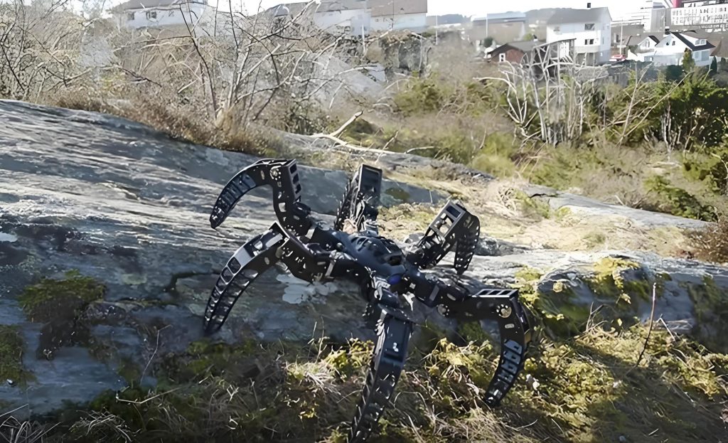
The true test of the bionic robot’s capabilities, however, lies in rough terrain navigation. I created an uneven terrain model using sinusoidal functions to simulate natural variations. The terrain height \( z \) at coordinates \( (x, y) \) was defined as:
$$ z = A_{x1} \sin(2\pi f_{x1} x) + A_{x2} \sin(2\pi f_{x2} x) + A_{y1} \sin(2\pi f_{y1} y) + A_{y2} \sin(2\pi f_{y2} y) $$
with amplitudes \( A = 0.2 \) m and frequencies chosen to produce realistic bumps and dips over a 4 m × 2 m area. The bionic robot started on flat ground and transitioned onto this rough terrain at a desired speed of 0.4 m/s. Throughout the simulation, the terrain adaptation mechanism was active, adjusting the body posture based on estimated slopes. The bionic robot successfully traversed the terrain in 14 seconds, maintaining stability without falls or excessive slipping. The body pitch and roll angles closely followed the terrain inclinations, with errors less than 0.05 radians. The foot forces remained consistent, with no abrupt spikes, indicating effective shock absorption. For instance, the vertical force on each foot varied between 300 N and 500 N, but the transitions were gradual, thanks to the compliant virtual model.
To quantify the bionic robot’s adaptation, I recorded the terrain angles and the corresponding body angles during the walk. The following table shows a sample of these values at different time intervals.
| Time (s) | Terrain Pitch (°) | Body Pitch (°) | Terrain Roll (°) | Body Roll (°) |
|---|---|---|---|---|
| 3.0 | 5.2 | 5.0 | -3.1 | -3.0 |
| 5.5 | -4.8 | -4.5 | 6.3 | 6.1 |
| 8.0 | 2.1 | 2.0 | -5.7 | -5.5 |
| 11.0 | -6.5 | -6.2 | 4.2 | 4.0 |
The close match between terrain and body angles underscores the efficacy of the adjustment strategy. Moreover, the bionic robot’s energy consumption, estimated from joint torque outputs, remained within acceptable limits, suggesting that this compliant gait is also efficient. These results collectively demonstrate that the bionic robot can handle significant terrain irregularities with grace and robustness, a key milestone for real-world deployment.
In conclusion, the compliant gait generation method based on virtual modeling offers a powerful solution for bionic robots to navigate rough terrain. By abstracting the bionic robot’s dynamics into spring-damper-mass systems, I have created a control framework that is both intuitive and effective. The virtual forces capture high-level locomotion goals, while the force distribution and joint torque conversion ensure precise low-level execution. Incorporating terrain feedback for body posture adjustment further enhances the bionic robot’s adaptability, allowing it to maintain stability on slopes and uneven surfaces. Simulation results on both flat and rough terrain validate the method, showing smooth force profiles, minimal body oscillations, and successful traversal of challenging landscapes. This approach aligns with bionic principles, mimicking the compliance and adaptability of biological organisms, and it paves the way for more advanced bionic robots capable of operating in diverse environments. Future work may involve implementing this control on physical bionic robot prototypes, exploring learning algorithms to optimize virtual parameters, and extending the method to other gaits like galloping. As bionic robots continue to evolve, such compliant control strategies will be integral to their success in applications ranging from search and rescue to planetary exploration.
The journey of developing this bionic robot has reinforced the importance of bio-inspiration in robotics. By studying how animals achieve smooth locomotion, we can engineer machines that not only replicate but also enhance natural capabilities. The bionic robot, with its compliant gait, represents a step toward more autonomous and resilient robotic systems. I believe that continued research in this direction will unlock new possibilities for bionic robots, making them indispensable partners in tackling complex tasks. Whether traversing rocky mountains or aiding in disaster response, the bionic robot equipped with adaptive compliance will stand as a testament to the synergy between biology and engineering.