
The pursuit of reliable and precise automation has positioned the RV (Rotate Vector) reducer as a cornerstone of modern robotics and high-precision machinery. As the core transmission component within industrial robot joints, the performance and longevity of the RV reducer directly dictate the operational reliability and precision retention of the entire system. Despite its widespread adoption and critical role, in-depth research specifically targeting the lifespan prediction and verification of RV reducers remains relatively scarce compared to more conventional gear units. Existing methodologies for traditional spur or worm gear reducers are insufficient due to the RV reducer’s inherent complexity, involving multi-tooth simultaneous engagement, high precision components, and a compact two-stage cycloidal-pin gear and planetary gear train structure. This article addresses this gap by establishing a theoretical framework for RV reducer life calculation, grounded in fundamental fatigue theories, and validates this framework through meticulously designed accelerated life testing. The development of a robust, practical lifespan model is paramount for design optimization, maintenance scheduling, and ensuring the long-term reliability of robotic systems.
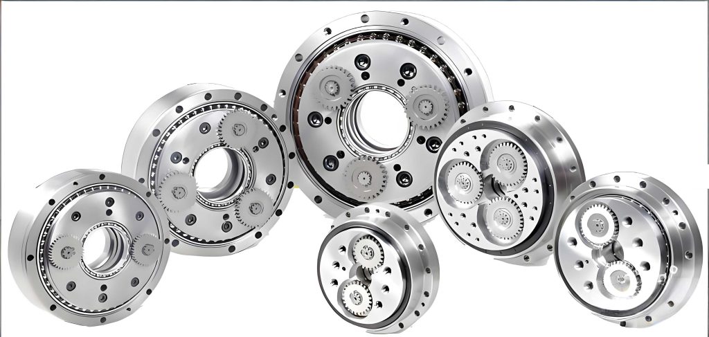
The operational principle of an RV reducer is key to understanding its lifespan challenges. The first stage typically consists of a planetary gear train, providing initial speed reduction. The second, crucial stage employs a cycloidal disc (or a pair of phase-shifted discs) meshing with a ring of stationary pin gears. This cycloidal-pin engagement, characterized by multi-tooth contact, is responsible for the high reduction ratio, high torsional stiffness, and compactness. However, this very mechanism subjects internal components, particularly the bearings supporting the crankshafts that drive the cycloidal discs, to complex and significant loading. The lifespan of the entire RV reducer assembly is often not limited by the gear teeth but by the fatigue life of these critical bearing elements operating under high load and relatively high rotational speed within the reducer’s compact housing.
Theoretical Foundation for RV Reducer Life Calculation
Predicting the lifespan of an RV reducer necessitates a foundation in material fatigue theory, as its failure typically stems from the fatigue of loaded components like bearings under cyclical stresses. The fundamental relationship between applied stress and the number of cycles to failure is described by the S-N curve (Stress-Number of cycles). For metallic components, this relationship in the finite life region can be expressed as a power law:
$$ \sigma^m N = \text{const} $$
where \(\sigma\) is the applied stress, \(N\) is the number of cycles to failure, and \(m\) is a material exponent. Since stress is proportional to applied force \(F\) or torque \(T\) in many mechanical elements, this can be adapted to:
$$ F^{m’} N = C \quad \text{or} \quad T^{m’} N = C $$
where \(m’\) is a component-specific exponent. This implies that for a given component, the permissible number of cycles is inversely proportional to the applied load raised to a power. For two different load conditions \(i\) and \(j\) on the same component, the relationship is:
$$ \left( \frac{F_i}{F_j} \right) = \left( \frac{N_j}{N_i} \right)^{1/m’} \quad \text{or} \quad \left( \frac{T_i}{T_j} \right) = \left( \frac{N_j}{N_i} \right)^{1/m’} $$
In practical operation, an RV reducer is subjected to a spectrum of varying loads over time. To assess the cumulative damage under such variable loading, Miner’s linear cumulative damage rule is employed. This rule postulates that failure occurs when the sum of the cycle ratios for each stress level equals unity. If a component experiences a series of torques \(T_1, T_2, …, T_n\) for corresponding cycles \(n’_1, n’_2, …, n’_n\), and the cycles to failure at these torque levels are \(N_1, N_2, …, N_n\), then failure is predicted when:
$$ \sum_{i=1}^{n} \frac{n’_i}{N_i} = 1 $$
Combining this with the power law relationship \(T^{m’}_i N_i = T^{m’}_0 N_0\) for a reference torque \(T_0\), we derive the equivalent life at the reference condition:
$$ N_0 = \sum_{i=1}^{n} \left( \frac{T_i}{T_0} \right)^{m’} n’_i $$
Since the total number of cycles \(N\) is related to operating time \(t\) and rotational speed \(n\) by \(N = n \cdot t\), the equivalent life in hours at the rated condition (speed \(n_0\), torque \(T_0\)) is:
$$ t_0 = \sum_{i=1}^{n} \left( \frac{T_i}{T_0} \right)^{m’} \left( \frac{n_i}{n_0} \right) t_i $$
If the RV reducer operates under a constant set of conditions \((T_a, n_a)\) until failure, its life \(t_a\) can be related to the rated life \(t_0\) by simplifying the above equation:
$$ t_a = t_0 \times \left( \frac{n_0}{n_a} \right) \times \left( \frac{T_0}{T_a} \right)^{p} $$
where \(p\) is the lifetime exponent, equivalent to \(m’\). This forms the fundamental lifespan formula for an RV reducer. However, actual operating conditions introduce factors that can accelerate fatigue. Therefore, an operational condition factor \(\alpha\) is introduced to account for lubrication effectiveness, contamination, temperature, and load distribution. The refined formula becomes:
$$ L_h = t_0 \times \left( \frac{N_0}{N_a} \right) \times \left( \frac{T_0}{T_a} \right)^{p} \times \alpha $$
Here, \(L_h\) represents the calculated life in hours, \(N_0\) and \(T_0\) are the rated speed and torque, \(N_a\) and \(T_a\) are the average operational speed and torque, and \(\alpha\) is typically chosen between 0.9 (for harsh conditions like poor lubrication or high temperature >40°C) and 1 (for ideal conditions).
The Critical Role of Needle Roller Bearings in RV Reducer Lifespan
Within the intricate assembly of an RV reducer, the needle roller bearings mounted on the crankshafts are frequently identified as the life-limiting components. These bearings, located between the cycloidal disc and the crankshaft’s taper roller bearing, directly support the load transmitted from the cycloidal-pin mesh. They operate at high relative speeds and under significant radial loads, making their fatigue life paramount. Consequently, the lifespan of the entire RV reducer can be effectively modeled based on the calculated life of these critical needle roller bearings.
The basic rating life \(L_{10}\) for a rolling bearing, representing the life in millions of revolutions that 90% of a group of identical bearings will exceed, is given by the ISO 281 standard:
$$ L_{10} = \left( \frac{C_r}{P_r} \right)^q $$
where \(C_r\) is the basic dynamic load rating, \(P_r\) is the equivalent dynamic radial load, and \(q\) is the life exponent (10/3 for roller bearings, 3 for ball bearings). For a needle roller bearing, the basic dynamic load rating \(C_r\) can be calculated using its specific geometry:
$$ C_r = b_m \cdot f_c \cdot (i \cdot L_{we} \cdot \cos\alpha)^{7/9} \cdot Z^{3/4} \cdot D_{we}^{29/27} $$
The parameters in this equation are defined in the following table:
| Symbol | Description | Typical Value/Note |
|---|---|---|
| \(b_m\) | Rating factor for material and manufacturing | 1.1 for contemporary roller bearings |
| \(f_c\) | Factor dependent on bearing geometry and accuracy | Obtained from manufacturer tables based on \(D_{pw}\) and \(D_{we}\) |
| \(i\) | Number of rows of rollers | Usually 1 for crankshaft needle bearings |
| \(\alpha\) | Nominal contact angle | 0° for radial needle bearings |
| \(L_{we}\) | Effective length of the roller | Measured value |
| \(Z\) | Number of rollers | Counted or from specification |
| \(D_{we}\) | Effective diameter of the roller | Measured value |
| \(D_{pw}\) | Pitch diameter of the roller set | \(D_{pw} \approx (Bore Diameter + Outer Diameter)/2\) |
The radial load \(F_r\) on the needle roller bearing originates from the output torque. Through force analysis of the cycloidal disc, this load can be derived as:
$$ F_r = \frac{1}{M} \cdot \frac{T_m}{R} \cdot 1000 $$
where \(T_m\) is the output torque of the RV reducer in Nm, \(R\) is the distance from the center of the cycloidal disc to the center of its bearing bore (in mm), and \(M\) is a load-sharing factor related to the number of crankshafts (typically 2 for RV-20E/40E models, leading to \(M=4\) considering two bearing positions per crankshaft and two cycloidal discs).
The rotational speed of the crankshaft bearing \(n’\) is significantly higher than the output speed \(n_{out}\) due to the reduction ratio. For an RV reducer with a reduction ratio \(i_{RV}\), the crankshaft speed is \(n’ \approx n_{out} \cdot i_{RV} / (1 + Z_p/Z_c)\) where \(Z_p\) is the number of pins and \(Z_c\) is the number of lobes on the cycloidal disc. A common approximation is \(n’ \approx n_{out} \cdot (i_{RV} – 1)\).
Combining these equations, the \(L_{10h}\) life in hours for the needle roller bearing is:
$$ L_{10h} = \frac{10^6}{60 \cdot n’} \left( \frac{C_r}{F_r} \right)^{10/3} $$
Substituting for \(F_r\) and \(n’\), and incorporating the overall transmission efficiency \(\eta\) of the RV reducer to account for internal losses affecting the load seen by the bearing, we arrive at a formula that links RV reducer operational parameters directly to bearing life:
$$ L_{10h} = \frac{10^6}{60 \cdot n_{out} \cdot (i_{RV}-1)} \left( \frac{C_r \cdot M \cdot R}{T_m \cdot 1000 / \eta} \right)^{10/3} $$
This calculation yields a baseline life \(t_0\) for the bearing under rated conditions. Observing that the exponent \(q\) for roller bearings is 10/3, and recognizing that the needle bearing life is the dominant constraint, we can set the exponent \(p\) in the general RV reducer life formula to 10/3. Thus, the final practical formula for estimating the \(L_{10h}\) life of an RV reducer becomes:
$$ L_h = K_0 \times \left( \frac{N_0}{N_a} \right) \times \left( \frac{T_0}{T_a} \right)^{10/3} \times \alpha $$
Here, \(K_0\) represents the rated lifespan in hours provided by the manufacturer under rated conditions \((N_0, T_0)\). This formula provides engineers with a direct method to estimate life under different operating conditions based on the manufacturer’s baseline rating.
Numerical Life Calculation for an RV-40E-121 Reducer
To demonstrate the application of the derived lifespan model, a theoretical calculation is performed for an RV-40E-121 type reducer. The rated parameters and key measured dimensions are summarized below.
| Parameter | Symbol | Value | Source/Note |
|---|---|---|---|
| Rated Output Torque | \(T_0\) | 412 Nm | Manufacturer Specification |
| Rated Output Speed | \(N_0\) | 15 rpm | Manufacturer Specification |
| Rated Lifespan | \(K_0\) (Target) | 6000 hours | Manufacturer Claim (Nabtesco) |
| Distance (Disc Center to Bearing Bore) | \(R\) | 36 mm | Measured via CMM |
| Load Sharing Factor | \(M\) | 4 | For RV-40E (2 crankshafts, 2 discs) |
| Transmission Efficiency | \(\eta\) | 0.75 | Calculated from performance tables |
| Reduction Ratio | \(i_{RV}\) | 121 | Model Designation |
| Operational Condition Factor | \(\alpha\) | 1 | Assumed ideal for baseline calculation |
| Dimension | Symbol | Value (mm) |
|---|---|---|
| Bore Diameter | – | 26 |
| Outer Diameter | – | 36 |
| Roller Effective Length | \(L_{we}\) | 9 |
| Roller Diameter | \(D_{we}\) | 5 |
| Pitch Diameter | \(D_{pw}\) | 31 |
| Number of Rollers | \(Z\) | 14 |
Step 1: Calculate Radial Load on Bearing.
Using the output torque and geometry:
$$ F_r = \frac{1}{4} \cdot \frac{412 \text{ Nm}}{0.036 \text{ m}} \cdot 1000 \approx 2861 \text{ N} $$
This is the load assuming perfect load sharing and no losses. Accounting for transmission efficiency, the effective load on the bearing is higher: \(F_{r, eff} = F_r / \eta \approx 2861 / 0.75 \approx 3815 \text{ N}\).
Step 2: Calculate Basic Dynamic Load Rating \(C_r\).
First, determine \(f_c\) from standard tables for \(D_{pw}=31\)mm and \(D_{we}=5\)mm. A typical value for this size is approximately 88.5. Applying the formula:
$$ C_r = 1.1 \times 88.5 \times (1 \times 9 \times \cos 0^\circ)^{7/9} \times 14^{3/4} \times 5^{29/27} $$
$$ C_r \approx 1.1 \times 88.5 \times (9)^{7/9} \times 8.62 \times 6.33 $$
$$ C_r \approx 19999 \text{ N} $$
Step 3: Calculate Bearing Life and Derive \(K_0\).
The crankshaft speed \(n’\) is needed. For an RV-40E with a ratio of 121, \(n’ \approx 15 \times (121 – 1) / (1 + 40/39) \approx 15 \times 40 = 600\) rpm (a common approximation). Using the bearing life formula with effective load:
$$ L_{10h} = \frac{10^6}{60 \times 600} \left( \frac{19999}{3815} \right)^{10/3} $$
$$ L_{10h} \approx 27.78 \times (5.24)^{10/3} $$
$$ (5.24)^{10/3} = (5.24^{1/3})^{10} \approx (1.738)^{10} \approx 250 $$
$$ L_{10h} \approx 27.78 \times 250 \approx 6944 \text{ hours} $$
This calculated value of 6944 hours represents the theoretical \(K_0\) based solely on the needle bearing analysis under ideal conditions (\(\alpha=1\)). It compares to the manufacturer’s specified 6000-hour rating with a difference of approximately:
$$ \text{Difference} = \frac{|6944 – 6000|}{6000} \times 100\% \approx 15.7\% $$
This close correlation validates the approach of using the critical needle roller bearing’s life as a proxy for the overall RV reducer’s lifespan and provides a rational basis for the exponent \(p=10/3\) in the general life formula. For practical use, the rated life constant \(K_0\) can be taken as the manufacturer’s value, e.g., 6000 hours.
Design and Implementation of an Accelerated Life Test Platform
Verifying the lifespan of an RV reducer through normal operation is impractical due to the thousands of hours required. Accelerated life testing (ALT) is therefore essential. The principle is to subject the RV reducer to conditions more severe than rated (typically higher load) to induce failure in a much shorter time, then use the lifespan model to correlate the accelerated life back to expected life under normal conditions.
A dedicated ALT platform was designed with the following key components and objectives:
- Loading Mechanism: A rotating arm with adjustable counterweights applies a constant, high bending moment and torque to the RV reducer output flange, simulating a severe robotic arm condition.
- Drive System: A servo motor provides precise input speed and torque control.
- Monitoring System: High-precision displacement sensors (e.g., capacitive or LVDT) continuously measure the angular backlash or positional repeatability of the output. Temperature sensors monitor housing temperature. Vibration sensors may also be used.
- Data Acquisition: A real-time system logs sensor data, tracking the degradation of positional precision over time.
The test is considered complete when the RV reducer’s measured performance (e.g., positional repeatability) degrades beyond a specified failure threshold (e.g., exceeding 1 arc-minute).
Accelerated Life Test Procedure and Results Analysis
An RV-20E-121 reducer was selected for the accelerated test. The test conditions were designed to significantly reduce the expected time to failure based on the life formula with \(p=10/3\).
| Parameter | Rated Condition | Accelerated Test Condition |
|---|---|---|
| Output Torque (\(T\)) | 167 Nm (\(T_0\)) | 318.5 Nm (\(T_a\)) |
| Output Speed (\(N\)) | 15 rpm (\(N_0\)) | 15 rpm (\(N_a\)) |
| Rated Life (\(K_0\)) | 6000 hours | – |
| Condition Factor (\(\alpha\)) | 1 (ideal) | 0.9 (poor lubrication, T>40°C) |
Theoretical Prediction for Test Duration:
Applying the lifespan formula to predict the time to failure under accelerated test conditions (\(L_h = t_{test}\)):
$$ t_{test} = 6000 \times \left( \frac{15}{15} \right) \times \left( \frac{167}{318.5} \right)^{10/3} \times 0.9 $$
First, calculate the torque ratio exponent:
$$ \left( \frac{167}{318.5} \right)^{10/3} = (0.524)^{10/3} $$
$$ 0.524^{1/3} \approx 0.806, \quad \text{then } 0.806^{10} \approx 0.116 $$
$$ t_{test} \approx 6000 \times 1 \times 0.116 \times 0.9 \approx 626 \text{ hours} $$
Thus, the theoretical prediction suggested failure would occur after approximately 626 hours of continuous testing under these accelerated conditions.
Test Execution and Results:
The RV reducer was run continuously on the ALT platform. Key data logged included housing temperature and output positional accuracy. The temperature profile showed a rapid rise from ambient (21°C) to around 45°C in the first 120 minutes, stabilizing with minor fluctuations around 46°C thereafter, confirming the “harsh condition” assumption (\(\alpha=0.9\)).
The most critical metric was the progressive loss of positioning accuracy. The data revealed a distinct three-phase pattern:
1. Initial Run-in/Wear-in (0-100 hours): A relatively rapid decline in accuracy (approx. 0.05 mm loss) as surfaces mate and initial wear occurs.
2. Stable Wear (100-580 hours): A period of steady, very gradual accuracy loss (approx. 0.03 mm over 480 hours), indicative of normal, predictable wear.
3. Failure Onset (580+ hours): A sudden, sharp decline in accuracy (approx. 0.04 mm step loss) with no recovery, indicating the onset of catastrophic failure modes such as spalling in bearings or severe wear in the cycloid-pin mesh. The cumulative error at this point exceeded the 1 arc-minute specification.
The test was stopped at approximately 580 hours when the failure threshold was clearly breached.
Verification of Theory:
Comparing the experimental result (580 hours) with the theoretical prediction (626 hours):
$$ \text{Error} = \frac{|580 – 626|}{626} \times 100\% \approx 7.3\% $$
This close agreement (within 8%) strongly validates the proposed RV reducer lifespan calculation formula with exponent \(p=10/3\) and the use of an operational condition factor \(\alpha\). Furthermore, it demonstrates the profound effectiveness of the accelerated life test platform. By applying a load roughly 1.9 times the rated torque, the test condensed nearly 6000 hours of rated operation into just 580 test hours, achieving an acceleration factor of approximately 10.3.
Discussion and Conclusion
This comprehensive analysis bridges the gap between theoretical lifespan modeling and practical validation for RV reducers. The derived lifespan formula, $$ L_h = K_0 \times (N_0/N_a) \times (T_0/T_a)^{10/3} \times \alpha $$, provides a practical and theoretically sound tool for engineers. Its foundation in the fatigue life of the critical needle roller bearing is justified by the mechanical design and failure mode analysis of the RV reducer. The exponent of 10/3 is directly adopted from the standard roller bearing life calculation, establishing a coherent link between component and system reliability.
The numerical case study on the RV-40E-121 reducer showed that a first-principles calculation focusing on the needle bearing yields a life estimate within 16% of the manufacturer’s published rating. This discrepancy is reasonable considering the simplifications in the load-sharing model and the exclusion of other potential failure modes. For practical application, using the manufacturer’s \(K_0\) value within this formula is recommended for different operating conditions.
The successful design and implementation of the accelerated life test platform represent a significant contribution to RV reducer quality assurance and research. The platform enables:
- Rapid Life Validation: Qualifying a unit’s lifespan in weeks instead of years.
- Design Comparison: Objectively comparing different designs or manufacturing batches.
- Failure Mode Analysis: Studying degradation patterns and identifying weak points.
- Model Calibration: Providing empirical data to refine theoretical models.
The excellent correlation (within 8%) between the predicted and actual accelerated test life for the RV-20E-121 unit provides robust empirical validation for the proposed lifespan model. It confirms that under carefully controlled and understood accelerated conditions, the failure mechanics scale according to the predicted power law.
In conclusion, the integration of a theoretically derived lifespan model based on critical component analysis with a physically realized accelerated testing methodology offers a complete framework for addressing the longevity and reliability of RV reducers. This framework is essential for advancing the state-of-the-art in precision robotics, ensuring that these core components meet the demanding lifecycle requirements of modern industrial applications. Future work may focus on further refining the operational condition factor \(\alpha\) with more granular parameters for lubrication, contamination, and temperature, and on extending the model to account for dynamic load spectra more complex than the constant load used in this derivation and test.