
The precision of power transmission in industrial and agricultural machinery is paramount for ensuring operational reliability, efficiency, and longevity. Among the various components that constitute these systems, the reducer plays a critical role in modulating speed and torque. A standout design in this category is the Rotary Vector (RV) reducer, renowned for its high reduction ratio, compact structure, robust load-bearing capacity, and superior torsional rigidity. This has led to its widespread adoption in demanding applications such as robotic arms, precision machine tools, and specialized agricultural equipment like slot-type compost turners. In these contexts, the RV reducer’s performance directly influences the accuracy and smoothness of the turning or positioning operations. However, the final transmission accuracy of an assembled rotary vector reducer is not solely determined by the theoretical design of its gears but is a cumulative outcome of various geometric and assembly deviations inherent in its constituent parts. This analysis delves deeply into the mechanisms through which these part-level deviations propagate through the assembly, ultimately affecting the system-level transmission error. We focus on establishing a theoretical framework for modeling this deviation propagation, which is crucial for guiding precision manufacturing and assembly processes.
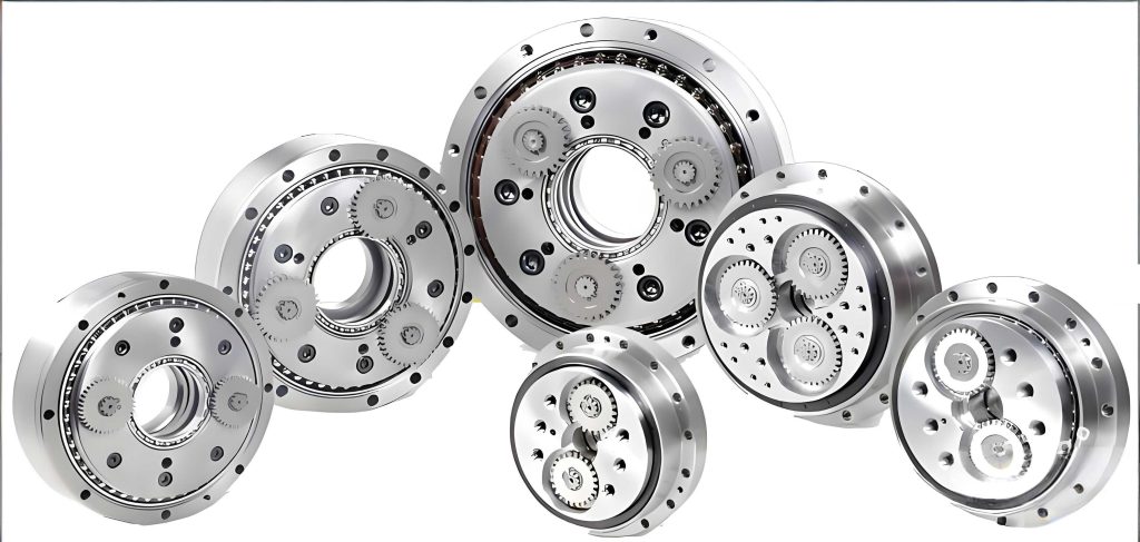
The core architecture of a typical rotary vector reducer consists of a two-stage planetary gear system. The primary reduction stage employs a standard involute planetary gear train. The sun gear, connected to the input shaft, drives multiple planet gears housed within a carrier. This stage provides the initial speed reduction. The secondary and defining stage is a cycloidal-pinwheel (or摆线针轮) mechanism. The planet carrier from the first stage is connected to eccentric crankshafts. These crankshafts drive cycloidal discs, which mesh with a stationary ring of pinwheels (or pins) housed in the casing. The unique motion of the cycloidal disc—simultaneous revolution and reverse rotation—is extracted by an output mechanism (often a wobble plate or pin), resulting in the final, high-ratio output. The overall reduction ratio $i_{total}$ of the rotary vector reducer is a product of the ratios from both stages:
$$ i_{total} = i_{stage1} \times i_{stage2} = (1 + \frac{Z_{ring1}}{Z_{sun}}) \times (\frac{Z_{pin}}{Z_{pin} – Z_{cycloid}}) $$
where $Z_{sun}$, $Z_{ring1}$, $Z_{cycloid}$, and $Z_{pin}$ are the tooth numbers of the sun gear, first-stage ring gear (often the housing), cycloidal disc, and pinwheel, respectively.
Taxonomy and Characterization of Deviation Sources in Rotary Vector Reducers
To systematically analyze error propagation, it is essential to first classify the sources of deviation within the rotary vector reducer assembly. These deviations arise from limitations in manufacturing processes and assembly operations. For the purpose of constructing a propagation model, we categorize deviations into three fundamental types, as summarized in Table 1.
| Deviation Class | Symbol | Description | Typical Examples in RV Reducer |
|---|---|---|---|
| Geometric Position Deviation | $E_1$ or $\Delta D$ | Deviations in the ideal location or orientation of a feature’s axis or plane. | Parallelism error between input shaft axis and crankshaft axis; coaxiality error of bearing bores. |
| Geometric Form Deviation | $E_2$ or $\Delta d$ | Deviations in the perfect shape or contour of a feature itself. | Profile error of cycloidal tooth flank; flatness error of a mounting face; roundness error of a shaft journal. |
| Assembly Position Deviation | $E_3$ or $\Delta T$ | Deviations introduced during the joining of parts, relative to their intended mating position. | Positional shift during press-fitting of bearings; backlash or misalignment in gear meshes due to mounting. |
In the static analysis of an assembled rotary vector reducer, the cumulative effect of these coupled deviations from all components determines the final positional error of the output flange relative to the input shaft, which is a critical measure of transmission accuracy. The assembly position deviation $E_3$ can often be modeled as a corrective term applied to the geometric position deviations $E_1$.
Mechanism of Deviation Propagation Through Assembly Interfaces
The propagation of deviations occurs at the interfaces where components mate. The nature of this mating defines how a deviation on one part influences the position and orientation of the subsequent part. We model components using functional geometric (FG) elements (e.g., a cylindrical surface for a bearing seat, a plane for a face) and datum/ideal geometric (DG) elements (e.g., a theoretical axis). A deviation is associated with an FG element.
The mating relationship between two parts can be classified based on the types of geometries involved, as shown in Table 2. This classification directly influences which deviation sources are active at the interface.
| Mating Type | Description | Active Deviation Sources |
|---|---|---|
| Mgg (FG-FG) | Both mating geometries are functional (deviated) geometries. | $\Delta d_1$, $\Delta d_2$, $\Delta T_2$ (All three sources interact). |
| MgD (FG-DG) | One mating geometry is functional, the other is a datum/ideal geometry. | $\Delta d_1$, $\Delta T_2$ (The DG has no form error). |
| MDD (DG-DG) | Both mating geometries are datum/ideal geometries. | $\Delta T_2$ (Only assembly positioning matters). |
Furthermore, the state of the fit—whether it is a clearance fit or an interference/non-clearance fit—governs the continuity of deviation accumulation. In a non-clearance fit (Mf), deviations from the first part directly cause a compensatory shift in the mated second part, leading to continuous accumulation. In a clearance fit (Mj), the clearance can interrupt the direct propagation chain; the final position of the second part is more dominantly governed by its own assembly position deviation $\Delta T_2$, effectively resetting the accumulation from that point. The statistical model for the resultant mating deviation $\Delta M$ for different combinations is critical for propagation analysis.
Directed Graph Representation of Deviation Flow
A powerful method to visualize and compute the propagation of deviations through a complex assembly like the rotary vector reducer is the Directed Deviation Graph (DDG). In this graph, nodes represent the functional geometric features of parts, and directed edges represent the transfer of deviation from one feature to another through a mating relationship.
The deviation on a feature can be represented by a six-dimensional statistical vector describing its small-displacement torsor (SDT):
$$ \mathbf{E_i} = [\Delta u, \Delta v, \Delta w, \Delta \alpha, \Delta \beta, \Delta \gamma]^T $$
where $\Delta u, \Delta v, \Delta w$ represent small linear displacements along the x, y, z axes, and $\Delta \alpha, \Delta \beta, \Delta \gamma$ represent small rotational deviations about these axes, all defined in a common coordinate system.
Assuming each component of the deviation vector follows a normal distribution, the multivariate statistical model for a deviation source is:
$$ f(\mathbf{E_i}) = (2\pi)^{-3} (\det \mathbf{P})^{-1/2} e^{[-\frac{1}{2}(\mathbf{E_i} – \boldsymbol{\mu})^T \mathbf{P}^{-1} (\mathbf{E_i} – \boldsymbol{\mu})]} $$
where $\boldsymbol{\mu} = (\mu_1, \mu_2, \mu_3, \mu_4, \mu_5, \mu_6)$ is the mean vector, and $\mathbf{P}$ is the 6×6 covariance matrix with elements $S_{ij}$.
For a planar surface feature with flatness tolerance $t$, the deviation domain can be characterized. If the surface lies in the XY-plane, the primary deviations are out-of-plane translation ($\Delta w$) and tilts ($\Delta \alpha, \Delta \beta$). The maximum values, considering a rectangular surface of length $L_1$ and width $W_1$, are:
$$ \max(\Delta w) = t, \quad \max(\Delta \alpha) = \frac{2t}{L_1}, \quad \max(\Delta \beta) = \frac{2t}{W_1}, \quad \Delta u=\Delta v=\Delta \gamma=0 $$
The mean vector is then $\boldsymbol{\mu} = (0, 0, t/2, t/L_1, t/W_1, 0)$. The constraints for a point on the surface are:
$$ \Delta w + \frac{|\Delta \alpha| L_1}{2} + \frac{|\Delta \beta| W_1}{2} \le t $$
To evaluate the impact of this plane’s deviation on a mating cylindrical feature (like a shaft), the deviations are transformed to the axis location. If $C_{11}$ is the radius at which the angular deviation acts, the equivalent linear and angular deviation vectors influencing the axis are:
$$ \mathbf{U_{axis}} = [0, 0, \Delta w, \Delta \alpha \cdot C_{11}, \Delta \beta \cdot C_{11}, 0]^T $$
$$ \mathbf{u_{axis}} = [0, 0, \Delta w/C_{11}, \Delta \alpha, \Delta \beta, 0]^T $$
The resultant magnitude of deviation contribution can be assessed as a Euclidean norm, e.g., $E = \sqrt{W^2 + A^2 + B^2}$ for linear effects.
Case Study: Deviation Propagation Analysis of an RV-40E Type Rotary Vector Reducer
To apply the theoretical framework, we conduct a detailed case study on an RV-40E type rotary vector reducer, commonly used in medium-duty applications. The first step is to decompose the assembly into its core functional components along the power flow: Input Shaft, Planetary Gears (3), Crankshafts (3), Needle Roller Bearings, Cycloidal Discs (2), Pin Housing, and Output Flange. For each mating interface between these components, we identify the mating type (Mgg, MgD, MDD), fit state (Mf or Mj), and the relevant deviation parameters with their typical tolerance ranges. A subset of this analysis for key components is presented in Table 3.
| Component | Mating Interface | Type & State | Key Deviation Parameters & Typical Range (mm or rad) |
|---|---|---|---|
| Input Shaft | Gear mesh with Sun/Planet | Mgg, Mf | Tooth profile error $\Delta d_{11}$, $\Delta d_{12}$: ±0.0001 |
| Planetary Gear | Bore fit on Crankshaft | MgD, Mf | Bore position $\Delta D_{21x}$, Form $\Delta d_{21x}$: ±0.00015 |
| Crankshaft | Journal fit in Bearing | MgD, Mj | Journal axis $\Delta D_{31}$, Form $\Delta d_{31}$: ±0.0002; Assembly $\Delta T_{3}$ |
| Cycloidal Disc | Tooth mesh with Pins | Mgg, Mf | Cycloidal tooth profile $\Delta d_{cyclo}$, Eccentric bore position $\Delta D_{eco}$: ±0.0001 |
| Output Flange | Pin-slot mechanism with Disc | MgD, Mj | Slot position $\Delta D_{out}$, Assembly $\Delta T_{out}$: ±0.00025 |
Based on this interface analysis, a comprehensive Directed Deviation Graph for the entire RV-40E rotary vector reducer assembly is constructed. This graph maps all deviation sources ($\Delta d_i$, $\Delta D_i$, $\Delta T_i$) from Table 3 and connects them through edges representing the mating relations, clearly showing the convergence paths from input to output.
The total transmission deviation $\Delta E_{total}$ at the output is the sum of deviations propagated through the first and second stages, scaled by their respective kinematic transformation ratios ($i_1$, $i_2$).
$$ \Delta E_{total} = \Delta E_{stage1} \cdot i_2 + \Delta E_{stage2} $$
Expanding this, $\Delta E_{stage1}$ includes contributions from sun gear, planet gear, and initial crankshaft mounting deviations. $\Delta E_{stage2}$ aggregates a far more extensive set of deviations from crankshaft bearing seats, eccentric sections, cycloidal disc bores and teeth, pin housing, and the output mechanism. The mathematical formulation becomes a large sum of the six-dimensional deviation vectors from each source, transformed through their respective coordinate systems to the output point.
To solve this complex stochastic model, the Monte Carlo method is employed. Using MATLAB, thousands of virtual assemblies are simulated. In each simulation, every deviation parameter (e.g., $\Delta d_{11}$, $\Delta D_{31}$) is randomly sampled from its defined statistical distribution (e.g., normal distribution within its tolerance range). These sampled deviations are propagated through the directed graph model using the kinematic and mating constraints to compute the resultant output error $\Delta E_{total}$ for that virtual assembly. The statistical results from all simulations provide the probable range of the final transmission error.
The simulation results for the RV-40E rotary vector reducer indicate that the absolute value of the final angular transmission deviation typically falls within the range of 0.017 to 0.957 arc-minutes. This is within the common accuracy specification of 1 arc-minute for many industrial-grade rotary vector reducers. A key insight from the Monte Carlo analysis is the contribution breakdown between stages. As shown in Table 4, the second-stage cycloidal-pinwheel system contributes over 80% to the total output deviation on average, significantly more than the first planetary stage.
| Simulation Batch | Stage 1 (Planetary) Contribution | Stage 2 (Cycloidal) Contribution | Total Deviation (arc-min) |
|---|---|---|---|
| 1 | 21.6% | 78.4% | 0.42 |
| 2 | 2.2% | 97.8% | 0.78 |
| 3 | 2.8% | 97.2% | 0.65 |
| 4 | 15.8% | 84.2% | 0.31 |
| 5 | 12.3% | 87.7% | 0.53 |
| Mean | ~11.0% | ~89.0% | 0.54 |
Conclusion and Engineering Implications
This theoretical and simulation-based analysis provides a structured methodology for understanding and quantifying transmission deviation propagation in rotary vector reducers. The core findings are:
- Systematic Modeling is Essential: The transmission accuracy of an assembled rotary vector reducer is a system-level property emerging from the interaction of numerous part-level deviations. A directed graph model coupled with statistical methods like Monte Carlo simulation provides a powerful tool for predicting this accuracy.
- Second-Stage Dominance: For the studied RV-40E type and similar rotary vector reducer architectures, the cycloidal-pinwheel (second) stage is the dominant contributor to the overall transmission error. This is due to the larger number of sensitive interfaces (crankshaft bearings, eccentricities, cycloid-pin mesh, output pins) and the high kinematic gain of this stage.
- Guidance for Precision Manufacturing: The analysis directly informs manufacturing and quality control priorities. To enhance the overall accuracy of a rotary vector reducer, tightening tolerances on second-stage components—particularly the crankshaft eccentricity, cycloidal disc tooth profile and bore location, and pin housing bore positions—will yield the most significant improvement per unit cost compared to focusing on the first planetary stage.
- Application to Agricultural Machinery: For equipment like slot-type compost turners, where consistent and reliable motion is critical for efficient aeration and mixing, understanding the RV reducer’s error sources helps in selecting appropriate reducer grades and informs maintenance schedules. It also guides the development of more robust and accurate drive systems for organic waste processing, contributing to more efficient and environmentally sustainable agricultural practices.
In summary, mastering the deviation propagation mechanism within the rotary vector reducer is not merely an academic exercise but a practical necessity for advancing the design, manufacturing, and application of high-precision drive systems across industries, including modern precision agriculture.