
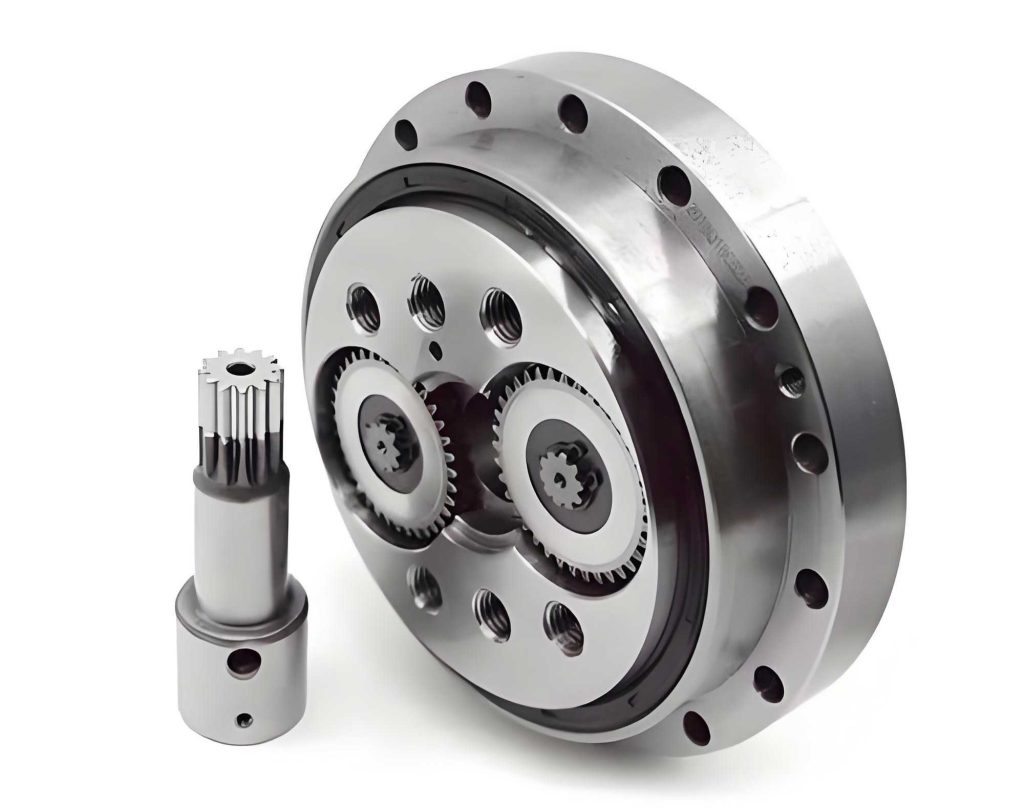
The RV reducer is a critical precision transmission component widely used in industrial robots and other high-end automated equipment. Its performance directly influences the positioning accuracy, motion smoothness, and operational stability of the entire system. The accurate acquisition of kinetic parameters, such as output torque, is fundamental for precise motion control, state monitoring, and health prognostics. However, signals measured from a RV reducer during operation are invariably contaminated by noise from various sources, including electrical interference from sensors and data acquisition systems, and mechanical vibrations from the transmission system itself. This noise obscures the true signal, leading to control inaccuracies and reduced system performance. Therefore, effective signal denoising is an essential pre-processing step for utilizing RV reducer data reliably.
Traditional frequency-domain filtering methods (e.g., low-pass filters) often struggle with non-stationary and non-linear signals commonly encountered in mechanical systems. Empirical Mode Decomposition (EMD) provides a powerful, adaptive alternative for processing such complex signals. The core idea of EMD-based denoising lies in decomposing the original signal into a series of Intrinsic Mode Functions (IMFs), which represent oscillatory components from high to low frequency. By identifying and processing IMFs dominated by noise differently from those containing useful information, one can reconstruct a cleaner signal.
This article presents a refined denoising strategy based on the EMD framework, specifically designed to handle the kinetic parameter signals from a RV reducer. The proposed method employs a dual-criterion approach to accurately categorize IMFs into three distinct groups and applies tailored processing to each, followed by a partial reconstruction to achieve superior noise suppression.
Mathematical Framework for the Denoising Algorithm
The Empirical Mode Decomposition (EMD) algorithm adaptively decomposes a signal \(x(t)\) into a finite number of oscillatory components called Intrinsic Mode Functions (IMFs), \(F_{IM,i}(t)\), and a residual trend \(r(t)\). This process can be expressed as:
$$x(t) = \sum_{i=1}^{L} F_{IM,i}(t) + r(t) = \sum_{i=1}^{L+1} F_{IM,i}(t)$$
where the residual \(r(t)\) is treated as the final IMF component. The fundamental challenge in EMD-based Part Reconstruction (EMD-PR) denoising is to correctly distinguish between noise-dominant, information-dominant, and mixed IMFs.
Criterion 1: Consecutive Mean Square Error (CMSE)
Noise components typically manifest in the lower-order (higher-frequency) IMFs. Their energy tends to decrease as the IMF order increases. The CMSE metric exploits this characteristic. Let \(\tilde{y}_k(t)\) represent the partial sum of IMFs from index \(k\) to the end:
$$\tilde{y}_k = \sum_{i=k}^{L+1} F_{IM,i}(t)$$
The CMSE between two consecutive partial sums is defined as:
$$ECMS(\tilde{y}_k, \tilde{y}_{k+1}) = \frac{1}{N}\sum_{j=1}^{N} [\tilde{y}_k(t_j) – \tilde{y}_{k+1}(t_j)]^2 = \frac{1}{N}\sum_{j=1}^{N} [F_{IM,k}(t_j)]^2$$
This is effectively the normalized energy of the \(k\)-th IMF. For primarily noisy IMFs, this energy decreases with increasing \(k\). The transition point \(M_1\), where the signal energy contribution begins to stabilize or increase due to the emergence of dominant information components, can be identified as the first local minimum of the CMSE sequence:
$$M_1 = \arg \,\text{first local min}_{1 \leq k \leq L} [ECMS(\tilde{y}_k, \tilde{y}_{k+1})]$$
IMFs with indices \(i < M_1\) are classified as noise-dominant IMFs.
Criterion 2: Signal Similarity via \(l_2\)-Norm of Probability Distributions
While CMSE effectively identifies the high-frequency noise floor, distinguishing between mixed and purely informational IMFs requires a different metric. Direct time-domain comparisons are sensitive to random fluctuations. A more robust method is to compare the probability density functions (PDFs) of the signals. The similarity between an IMF component \(S_1(t)=F_{IM,k}(t)\) and the original signal \(S_2(t)=x(t)\) can be quantified using the \(l_2\)-norm of the difference between their PDFs, \(P_{S_1}(y)\) and \(P_{S_2}(y)\):
$$L(S_1, S_2) = ||P_{S_1} – P_{S_2}||_2 = \left( \int_{-\infty}^{+\infty} [P_{S_1}(y) – P_{S_2}(y)]^2 \, dy \right)^{\frac{1}{2}}$$
A smaller \(l_2\)-norm indicates greater similarity in the statistical distribution. However, this metric is sensitive to both distribution shape and mean value. Lower-order (noisy) IMFs may have a small \(l_2\)-norm due to a near-zero mean, despite having a completely different shape from the original signal. Therefore, this criterion is applied selectively. After determining \(M_1\), we search for the index \(M_2\) among higher-order IMFs (\(k > M_1\)) where the dissimilarity is greatest. This point often marks a transition between mixed modes and the core informational mode. Formally, we define \(M_2\) as:
$$M_2 = \arg \max_{M_1 < k \leq L} [L(F_{IM,k}, x)]$$
IMFs with indices \(M_1 \leq i \leq M_2\) are classified as mixed IMFs, containing both noise and information. IMFs with indices \(i > M_2\) are classified as information-dominant IMFs.
| IMF Class | Index Range | Dominant Content | Processing Action |
|---|---|---|---|
| Noise-dominant | \(1 \leq i < M_1\) | Primarily high-frequency noise | Discard completely. |
| Mixed | \(M_1 \leq i \leq M_2\) | Mix of noise and signal information | Apply secondary denoising (e.g., Kalman filter). |
| Information-dominant | \(M_2 < i \leq L+1\) | Primarily the true kinetic signal | Retain without modification. |
Algorithm Framework for RV Reducer Signal Denoising
The complete denoising framework for signals from a RV reducer integrates the classification criteria and processing strategies. Ensemble EMD (EEMD) is employed to mitigate mode mixing, and mirror extension is used to suppress endpoint effects. The algorithm proceeds as follows:
- Decomposition: Apply EEMD to the raw kinetic parameter signal \(x(t)\) (e.g., torque) from the RV reducer to obtain IMFs \(F_{IM,i}(t)\).
- Noise Floor Identification: Calculate the CMSE for the IMF series. Determine the index \(M_1\) as the first local minimum of CMSE.
- Information Core Identification: Calculate the \(l_2\)-norm of the PDF between each IMF (for \(i > M_1\)) and the original signal. Determine the index \(M_2\) as the argument of the maximum value within this range.
- Targeted Processing:
- Discard IMFs for \(i = 1, …, M_1-1\).
- Apply a Kalman filter to each mixed IMF in the range \(i = M_1, …, M_2\). The Kalman filter is effective for smoothing linear-like signals with white noise.
- Retain the information-dominant IMFs for \(i = M_2+1, …, L+1\) unchanged.
- Partial Reconstruction: The denoised signal \(\hat{x}(t)\) is reconstructed by summing the processed components:
$$\hat{x}(t) = \sum_{i=M_1}^{M_2} F_{IM,i}^{Kalman}(t) + \sum_{i=M_2+1}^{L+1} F_{IM,i}(t)$$
Application to RV Reducer Torque Signals
Experimental Setup and Signal Characteristics
The proposed method was validated using experimental data from an RV40E RV reducer. The test platform measured input and output torque and speed under different input rotational speeds (1000 rpm, 2000 rpm, 3000 rpm) with a sampling frequency of 1000 Hz. While speed signals were relatively clean, torque signals exhibited significant contamination.
The input torque signal, primarily governed by the servo motor driver, was contaminated mainly by wide-band sensor noise. The output torque signal displayed a superposition of periodic fluctuations (inherent to the RV reducer‘s cyclic mechanical action) and substantial random noise, making accurate feature extraction challenging.
| Parameter | Value / Description |
|---|---|
| RV Reducer Model | RV40E |
| Input Speeds Tested | 1000, 2000, 3000 rpm |
| Sampling Frequency | 1000 Hz |
| Primary Noisy Signal | Input and Output Torque |
| Noise Sources | Sensor electronics, mechanical vibration |
Denoising Process and Results
The 3000 rpm condition is used as a detailed case study. The raw input and output torque signals were decomposed via EEMD. The CMSE and \(l_2\)-norm metrics were calculated for the resulting IMFs. For the input torque signal, the criteria yielded \(M_1 = 4\) and \(M_2 = 10\). For the output torque, \(M_1 = 4\) and \(M_2 = 9\). This confirmed the first few IMFs as noise, a middle set as mixed, and the final IMFs as carrying the core information or trend.
The mixed IMFs (indices \(M_1\) to \(M_2\)) were processed with a Kalman filter before reconstruction. The final denoised signals for both input and output torque at 3000 rpm showed a dramatic reduction in high-frequency noise while preserving the underlying trend and periodic characteristics, especially visible in the output torque’s harmonic fluctuation.
The process was repeated for the 1000 rpm and 2000 rpm datasets with equally effective results, demonstrating the robustness of the method across different operating conditions of the RV reducer.
Performance Evaluation
The effectiveness of the denoising algorithm was quantified using the Signal-to-Noise Ratio (SNR), calculated before and after processing. A significant improvement in SNR indicates successful noise suppression.
| Operating Condition | Input Torque SNR (dB) | Output Torque SNR (dB) | ||
|---|---|---|---|---|
| Original | Denoised | Original | Denoised | |
| 1000 rpm | 15.13 | 27.44 | 27.09 | 35.58 |
| 2000 rpm | 8.61 | 20.58 | 23.31 | 31.42 |
| 3000 rpm | 8.80 | 30.51 | 23.25 | 31.32 |
The results in Table 3 conclusively demonstrate the method’s efficacy. The SNR improved substantially for all test cases. Notably, the input torque signals, which had lower original SNRs (indicating stronger noise corruption), showed the most dramatic improvements. The output torque signals, which contained inherent periodic information from the RV reducer transmission, also saw significant noise reduction, making the harmonic components more distinct and usable for further analysis like error compensation or fault diagnosis.
Discussion on IMF Classification Metrics
The dual-criterion approach is crucial for accurate IMF classification. The CMSE metric effectively captures the energy decay of noise components but can be non-monotonic. Relying on the first local minimum is a pragmatic rule for identifying the noise floor threshold \(M_1\) for signals from a RV reducer.
The \(l_2\)-norm of PDFs provides a complementary, shape-sensitive measure. Its behavior requires careful interpretation. The initial rise in the \(l_2\)-norm for mid-range IMFs (from \(M_1\) to \(M_2\)) indicates these components have a statistical distribution increasingly different from both the pure noise and the final trend/information. This aligns with them being “mixed” modes. The subsequent drop for the highest-order IMFs (beyond \(M_2\)) confirms their high similarity to the core signal component, justifying their classification as information-dominant. This nuanced interpretation, guided by the sequential application of CMSE first, prevents misclassification that could occur using either metric alone.
Conclusion
Accurate kinetic parameter acquisition is vital for the high-performance operation of systems employing an RV reducer. The noise inherent in measurement signals poses a significant challenge. This article presented a sophisticated EMD-based denoising method tailored for this purpose. The key innovation lies in the use of two complementary metrics—Consecutive Mean Square Error (CMSE) and the \(l_2\)-norm of probability density functions—to classify EMD-derived IMFs into three categories: noise-dominant, mixed, and information-dominant.
By applying a targeted processing strategy (discarding, filtering with Kalman, and retaining) to each category and reconstructing the signal from the processed components, the method achieves highly effective noise suppression. Experimental validation on an RV40E RV reducer under various operating speeds confirmed the algorithm’s performance, with denoised torque signals showing markedly improved Signal-to-Noise Ratios. The denoised output torque signal, in particular, reveals the characteristic harmonic fluctuations of the RV reducer much more clearly, providing a cleaner data source for advanced control strategies, precision health monitoring, and dynamic performance evaluation of the transmission system.