
In the field of industrial automation and robotics, the demand for precise force measurement has led to significant advancements in sensor technology. Among various types, the six-axis force sensor stands out due to its ability to measure forces and moments along three orthogonal axes. This capability is crucial for applications such as robotic manipulation, aerospace testing, and automotive manufacturing. Traditional six-axis force sensors often rely on strain gauges or piezoelectric elements, but these can suffer from limitations like hysteresis, temperature sensitivity, and complex signal conditioning. In contrast, capacitive sensing offers advantages such as high sensitivity, low power consumption, and robustness to environmental factors. However, existing capacitive six-axis force sensors primarily utilize parallel-plate capacitors, which are prone to nonlinearities due to edge effects. To address this, we have developed a novel six-axis force sensor that combines two distinct capacitive effects: the edge effect of vertical plate capacitors and the variable gap effect of parallel-plate capacitors. This integration aims to reduce inter-dimensional coupling and improve overall accuracy. In this paper, we present the theoretical foundations, structural design, decoupling methodology, and experimental validation of this innovative six-axis force sensor.
The core principle of our six-axis force sensor lies in leveraging two capacitive mechanisms. The first is the variable gap parallel-plate capacitor effect, where the capacitance changes with the distance between two parallel plates. The capacitance \( C \) for an ideal parallel-plate capacitor is given by:
$$ C = \frac{\varepsilon S}{d} $$
where \( \varepsilon \) is the permittivity of the dielectric medium, \( S \) is the overlapping area of the plates, and \( d \) is the separation distance. When an external force causes a change \( \Delta d \) in the initial gap \( d_0 \), the capacitance change \( \Delta C \) can be expressed as:
$$ \Delta C = \frac{\varepsilon S}{d_0 – \Delta d} – C_0 $$
where \( C_0 = \frac{\varepsilon S}{d_0} \) is the initial capacitance. For small displacements where \( \Delta d \ll d_0 \), this can be linearized using a Taylor series expansion:
$$ \Delta C = C_0 \frac{\Delta d}{d_0} \left(1 + \frac{\Delta d}{d_0} + \left(\frac{\Delta d}{d_0}\right)^2 + \cdots \right) $$
Approximating to the first order, we get:
$$ \Delta C \approx C_0 \frac{\Delta d}{d_0} $$
The full-scale output \( Y_{\text{FS}} \) and linearity error \( \delta_L \) for a sensor based on this effect are derived as:
$$ Y_{\text{FS}} = C_0 \frac{\Delta d_{\text{max}}}{d_0} $$
$$ \delta_L \approx \frac{\Delta d_{\text{max}}}{d_0} \times 100\% $$
The sensitivity \( K_d \) is given by:
$$ K_d = \frac{C_0}{d_0} = \frac{\varepsilon S}{d_0^2} $$
This shows that sensitivity is proportional to the plate area \( S \) and inversely proportional to the square of the initial gap \( d_0 \).
The second mechanism is the vertical plate capacitor edge effect, which exploits the fringing fields between vertically aligned plates. For a vertical plate capacitor with plate width \( W \), height \( H \), and gap \( h \), the capacitance \( C \) is expressed as:
$$ C = \frac{4\varepsilon W}{\pi} \ln \frac{2H}{h} $$
When the gap changes by \( \Delta h \) from the initial value \( h_0 \), the capacitance change \( \Delta C \) becomes:
$$ \Delta C = -\frac{4\varepsilon W}{\pi} \ln \left(1 – \frac{\Delta h}{h_0}\right) $$
Expanding this using a Taylor series for \( \Delta h \ll h_0 \):
$$ \Delta C = \frac{4\varepsilon W}{\pi} \left( \frac{\Delta h}{h_0} + \frac{1}{2} \left( \frac{\Delta h}{h_0} \right)^2 + \frac{1}{3} \left( \frac{\Delta h}{h_0} \right)^3 + \cdots \right) $$
The linear approximation is:
$$ \Delta C \approx \frac{4\varepsilon W}{\pi h_0} \Delta h $$
The full-scale output and linearity error for this effect are:
$$ Y_{\text{FS}} = \frac{4\varepsilon W}{\pi h_0} \Delta h_{\text{max}} $$
$$ \delta_L \approx \frac{1}{2} \frac{\Delta h_{\text{max}}}{h_0} \times 100\% $$
with sensitivity \( K_{\text{vert}} \):
$$ K_{\text{vert}} = \frac{4\varepsilon W}{\pi h_0} $$
This indicates that sensitivity depends on the plate width \( W \) and inversely on the initial gap \( h_0 \). By combining these two effects, our six-axis force sensor achieves enhanced performance with reduced nonlinearities.
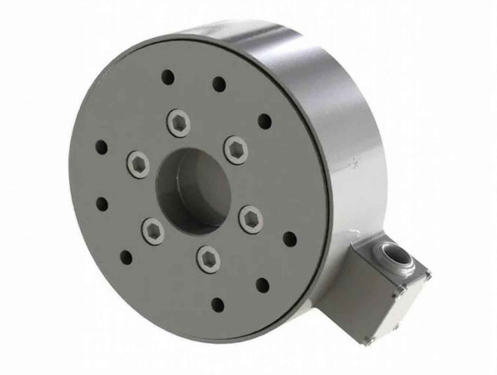
The structural design of our six-axis force sensor is optimized for manufacturability and minimal inter-dimensional coupling. It consists of three main layers: the body, the measurement layer, and the PCB layer. The body includes an outer ring, S-shaped deformation beams, a PCB mounting platform, and wiring holes. The S-shaped beams are critical as they amplify sensitivity and decouple forces by allowing controlled deformations. The measurement layer is divided into upper and lower sub-layers, which house the moving electrodes for both capacitor types. The PCB layer contains the static electrodes, detection circuitry, and a capacitance-to-digital converter chip that translates capacitive changes into digital signals.
In the measurement layer, we implement six differential capacitor pairs: three based on vertical plate edge effects and three on parallel-plate effects. The vertical plate capacitors are formed between moving electrodes on the measurement layer and static electrodes on the PCB, arranged in pairs (e.g., C1 and C2) to create differential capacitors CI, CIII, and CV. Similarly, the parallel-plate capacitors use moving electrodes on the upper and lower measurement layers opposing static electrodes on the PCB, forming differential pairs CII, CIV, and CVI. This differential configuration cancels common-mode noise and improves accuracy. The distribution of these capacitors is summarized in Table 1, which shows how each differential capacitor responds to applied forces and moments.
| Differential Capacitor | FX | FY | FZ | MX | MY | MZ |
|---|---|---|---|---|---|---|
| CI | Weak Increase | Strong Increase | No Change | Weak Decrease | Weak Increase | Strong Increase |
| CII | No Change | No Change | Strong Decrease | Strong Increase | No Change | No Change |
| CIII | Weak Increase | Strong Decrease | No Change | Weak Increase | Weak Increase | Strong Increase |
| CIV | No Change | No Change | Strong Decrease | Weak Decrease | Strong Decrease | No Change |
| CV | Strong Decrease | No Change | No Change | No Change | Weak Decrease | Strong Increase |
| CVI | No Change | No Change | Strong Decrease | Weak Decrease | Strong Increase | No Change |
When an external force is applied to the inner ring of the six-axis force sensor, it decomposes into six components: FX, FY, FZ, MX, MY, and MZ. The S-shaped beams deform, displacing the moving electrodes and altering the capacitances. The capacitance changes from the six differential pairs are recorded as a vector \( \Delta \mathbf{C} = [\Delta C_I, \Delta C_{II}, \Delta C_{III}, \Delta C_{IV}, \Delta C_V, \Delta C_{VI}]^T \). The relationship between the applied force vector \( \mathbf{F} = [F_X, F_Y, F_Z, M_X, M_Y, M_Z]^T \) and \( \Delta \mathbf{C} \) is modeled as:
$$ \mathbf{F} = \mathbf{T} \Delta \mathbf{C} $$
where \( \mathbf{T} \) is a 6×6 decoupling matrix. To compute \( \mathbf{T} \), we employ a least squares approach based on static calibration data. If we have \( n \) calibration points (with \( n > 6 \)), the force matrix \( \mathbf{F} \) (size 6×n) and capacitance change matrix \( \Delta \mathbf{C} \) (size 6×n) are used to solve:
$$ \mathbf{T} = \mathbf{F} (\Delta \mathbf{C}^T \Delta \mathbf{C})^{-1} \Delta \mathbf{C}^T $$
This method minimizes errors and ensures accurate decoupling even with noisy data. For our six-axis force sensor, we collected 66 calibration points to compute \( \mathbf{T} \), enhancing the precision of the decoupling matrix.
To validate the six-axis force sensor, we conducted static calibration experiments in a controlled environment free from vibrations and shocks. The calibration setup involved applying known forces and moments using weights and pulleys, with forces calculated as \( F = mg \) (where \( m \) is mass and \( g = 9.8 \, \text{m/s}^2 \)) and moments as \( M = mg \times L \) (with arm length \( L = 50 \, \text{mm} \)). The sensor’s range is defined in Table 2.
| Force/Moment | Range |
|---|---|
| FX, FY, FZ | 60 N |
| MX, MY, MZ | 3 N·m |
During calibration, we loaded each dimension from zero to full scale in increments, recording the capacitance changes. The decoupling matrix \( \mathbf{T} \) was derived using the least squares formula. For example, a subset of the force matrix \( \mathbf{F} \) and capacitance change matrix \( \Delta \mathbf{C} \) is shown below (simplified for illustration):
$$ \mathbf{F} = \begin{bmatrix}
9.8 & 0 & 0 & 0 & 0 & 0 \\
0 & 9.8 & 0 & 0 & 0 & 0 \\
0 & 0 & 9.8 & 0 & 0 & 0 \\
0 & 0 & 0 & 0.49 & 0 & 0 \\
0 & 0 & 0 & 0 & 0.49 & 0 \\
0 & 0 & 0 & 0 & 0 & 0.49 \\
\vdots & \vdots & \vdots & \vdots & \vdots & \vdots \\
58.8 & 0 & 0 & 0 & 0 & 0 \\
0 & 58.8 & 0 & 0 & 0 & 0 \\
0 & 0 & 58.8 & 0 & 0 & 0 \\
0 & 0 & 0 & 2.94 & 0 & 0 \\
0 & 0 & 0 & 0 & 2.94 & 0 \\
0 & 0 & 0 & 0 & 0 & 2.94 \\
\end{bmatrix} $$
$$ \Delta \mathbf{C} = \begin{bmatrix}
10.479 & 17.435 & 0.006 & -13.682 & 8.472 & 28.203 \\
-0.927 & 0.969 & 16.027 & 42.007 & -0.145 & -0.106 \\
10.651 & -17.937 & -0.079 & 14.983 & 8.507 & 28.489 \\
0.658 & -0.984 & 15.812 & -21.928 & -37.156 & -0.061 \\
-19.324 & 0.341 & 0.067 & -0.116 & -14.806 & 26.307 \\
-1.074 & -1.779 & 15.421 & -21.138 & 36.129 & 0.108 \\
\vdots & \vdots & \vdots & \vdots & \vdots & \vdots \\
64.433 & 111.767 & -0.133 & -84.181 & 51.334 & 178.586 \\
-3.315 & 2.266 & 95.807 & 254.687 & 1.208 & -0.812 \\
65.815 & -114.829 & -0.258 & 91.307 & 49.058 & 178.595 \\
2.157 & -3.780 & 95.268 & -132.623 & -236.691 & -0.032 \\
-118.253 & 2.091 & 0.519 & -0.995 & -94.756 & 167.283 \\
-5.769 & -8.834 & 92.751 & -128.053 & 239.285 & 1.069 \\
\end{bmatrix} $$
The computed decoupling matrix \( \mathbf{T} \) is:
$$ \mathbf{T} = \begin{bmatrix}
0.1546 & -0.0016 & 0.1498 & 0.0983 & -0.3245 & -0.0971 \\
0.2587 & 0.0060 & -0.2548 & -0.0567 & -0.0026 & -0.0622 \\
0.0133 & 0.2151 & -0.0051 & 0.2035 & -0.0085 & 0.2034 \\
-0.0002 & 0.0075 & 0.0003 & -0.0038 & 0.0000 & -0.0039 \\
0.0003 & 0.0001 & 0.0000 & -0.0063 & -0.0003 & 0.0064 \\
0.0055 & -0.0001 & 0.0054 & 0.0000 & 0.0060 & 0.0000 \\
\end{bmatrix} $$
To evaluate the decoupling performance of the six-axis force sensor, we use two error metrics: Type I error (relative error between applied and measured full-scale force) and Type II error (cross-coupling error). The decoupling error matrix \( \mathbf{E} \) is defined as:
$$ \mathbf{E} = \begin{bmatrix}
E_{F_X F_X} & E_{F_X F_Y} & E_{F_X F_Z} & E_{F_X M_X} & E_{F_X M_Y} & E_{F_X M_Z} \\
E_{F_Y F_X} & E_{F_Y F_Y} & E_{F_Y F_Z} & E_{F_Y M_X} & E_{F_Y M_Y} & E_{F_Y M_Z} \\
E_{F_Z F_X} & E_{F_Z F_Y} & E_{F_Z F_Z} & E_{F_Z M_X} & E_{F_Z M_Y} & E_{F_Z M_Z} \\
E_{M_X F_X} & E_{M_X F_Y} & E_{M_X F_Z} & E_{M_X M_X} & E_{M_X M_Y} & E_{M_X M_Z} \\
E_{M_Y F_X} & E_{M_Y F_Y} & E_{M_Y F_Z} & E_{M_Y M_X} & E_{M_Y M_Y} & E_{M_Y M_Z} \\
E_{M_Z F_X} & E_{M_Z F_Y} & E_{M_Z F_Z} & E_{M_Z M_X} & E_{M_Z M_Y} & E_{M_Z M_Z} \\
\end{bmatrix} $$
where diagonal elements represent Type I errors and off-diagonal elements represent Type II errors. For a full-scale applied force vector \( \mathbf{F}” \) and the corresponding measured force vector \( \mathbf{F} \) from decoupling, the errors are calculated as:
$$ \text{Type I Error} = \left| \frac{\text{Measured Force at Full Scale}}{\text{Applied Full-Scale Force}} \right| \times 100\% $$
$$ \text{Type II Error} = \left| \frac{\text{Measured Force in Other Direction}}{\text{Full-Scale Force in That Direction}} \right| \times 100\% $$
Based on our experiments, the decoupling error matrix for the six-axis force sensor is:
$$ \mathbf{E} = \begin{bmatrix}
0.19 & 0.02 & 0.04 & 0.19 & 0.36 & 0.33 \\
0.09 & 0.66 & 0.05 & 0.04 & 0.47 & 0.18 \\
0.14 & 0.05 & 0.10 & 0.27 & 0.14 & 0.12 \\
0.06 & 0.37 & 0.11 & 0.14 & 0.17 & 0.09 \\
0.04 & 0.06 & 0.08 & 0.14 & 0.39 & 0.02 \\
0.01 & 0.13 & 0.01 & 0.08 & 0.19 & 0.32 \\
\end{bmatrix} $$
This results in Type I errors of 0.19% for FX, 0.66% for FY, 0.10% for FZ, 0.14% for MX, 0.39% for MY, and 0.32% for MZ. The maximum Type II error is 0.47%, occurring when MY couples into FY. These low errors demonstrate that the six-axis force sensor has minimal inter-dimensional coupling and is highly decouplable.
In conclusion, we have successfully designed and validated a novel six-axis force sensor that integrates vertical plate capacitor edge effects and parallel-plate capacitor variable gap effects. The theoretical analysis confirms the linearity and sensitivity advantages of this dual approach. The layered structure, with S-shaped deformation beams, facilitates precise force measurement and reduces coupling. Through static calibration and least squares decoupling, we achieved a decoupling matrix that yields low Type I and Type II errors. This six-axis force sensor proves feasible for applications requiring high accuracy and minimal cross-talk, such as robotics and advanced manufacturing. Future work will focus on optimizing the design for broader dynamic ranges and environmental robustness.