
In recent years, with the rapid advancement of intelligent manufacturing, the Internet of Things, and robotics, the demand for high-precision force measurement has grown significantly. Among various force sensors, the six-axis force sensor stands out due to its ability to simultaneously measure three-dimensional forces and three-dimensional moments, making it indispensable in fields such as aerospace, automotive testing, biomechanics, and robotics. The six-axis force sensor is characterized by its high sensitivity, low inter-dimensional coupling, and mechanical overload protection, enabling it to convert force and moment components into electrical signals with micron-level accuracy. However, the design and calibration of a six-axis force sensor are challenging due to its nonlinear mechanical properties, multi-channel signal creep, cross-interference, and the complexity of joint loading calibration. This paper focuses on the design and static calibration of an orthogonal parallel six-axis force sensor, aiming to enhance measurement precision and support the development of intelligent equipment.
The six-axis force sensor is the highest-dimensional force sensor, providing comprehensive force information. It measures forces along the x, y, and z axes and moments around these axes in a Cartesian coordinate system. Originally developed for aerospace applications to assess aerodynamic characteristics like lift, drag, and moments, the six-axis force sensor has evolved into a critical component in robotics for force control and motion adjustment. For instance, in robotic operations, the six-axis force sensor allows the system to perceive and adjust to external forces, improving task accuracy. The dynamic performance of the six-axis force sensor varies based on application requirements, such as load capacity, installation environment, and communication protocols. Despite its advantages, the six-axis force sensor requires precise design and calibration to minimize errors, as even minor inaccuracies can lead to significant deviations in force measurement.
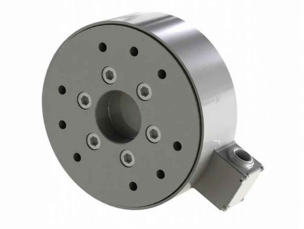
The orthogonal parallel six-axis force sensor operates on a unique structural principle. It consists of a base, a force measurement platform, and six force-sensing branches arranged in orthogonal horizontal and vertical configurations. The spatial coordinate definition of the six-axis force sensor is illustrated in the figure below, which shows the arrangement of the branches and the coordinate system. The horizontal branches measure forces in the x and y directions and the moment around the z-axis, while the vertical branches handle the force in the z direction and moments around the x and y axes. This orthogonal distribution enables effective decoupling of force and moment interactions, ensuring high accuracy. The six-axis force sensor can achieve measurement deviations within 0.3% FS under combined loading conditions, thanks to its optimized internal algorithms.
The mathematical model of the orthogonal parallel six-axis force sensor is derived from static equilibrium equations. Let $F$ represent the external force vector acting on the sensor, defined as $F = [F_x, F_y, F_z, M_x, M_y, M_z]^T$, where $F_x$, $F_y$, and $F_z$ are the force components along the x, y, and z axes, and $M_x$, $M_y$, and $M_z$ are the moment components around these axes. The axial forces in the six branches are denoted by the vector $f = [f_1, f_2, f_3, f_4, f_5, f_6]^T$. The relationship between the external forces and the branch forces is given by the equation:
$$ F = G \cdot f $$
Here, $G$ is a $6 \times 6$ influence coefficient matrix that depends on the geometry of the sensor, including the positions of the connection points between the branches and the platforms. For an orthogonal parallel six-axis force sensor, the matrix $G$ is constructed based on the vectors of the branches in the coordinate system. Let $b_i$ and $B_i$ represent the connection points on the force measurement platform and base for the i-th branch, respectively. The matrix $G$ is defined as:
$$ G = \begin{bmatrix}
\frac{\mathbf{b_1} – \mathbf{B_1}}{\|\mathbf{b_1} – \mathbf{B_1}\|} & \frac{\mathbf{b_2} – \mathbf{B_2}}{\|\mathbf{b_2} – \mathbf{B_2}\|} & \cdots & \frac{\mathbf{b_6} – \mathbf{B_6}}{\|\mathbf{b_6} – \mathbf{B_6}\|} \\
\frac{\mathbf{b_1} \times \mathbf{B_1}}{\|\mathbf{b_1} – \mathbf{B_1}\|} & \frac{\mathbf{b_2} \times \mathbf{B_2}}{\|\mathbf{b_2} – \mathbf{B_2}\|} & \cdots & \frac{\mathbf{b_6} \times \mathbf{B_6}}{\|\mathbf{b_6} – \mathbf{B_6}\|}
\end{bmatrix} $$
This matrix ensures that the branches are linearly independent, facilitating effective decoupling. For example, in a typical configuration, the vertical branches are arranged at 120-degree intervals around the center of the platform, and the horizontal branches are tangent to a central circle, also at 120-degree intervals. The specific form of $G$ for such a sensor can be simplified based on symmetry. Assuming a symmetric design with branch vectors aligned along orthogonal directions, the matrix $G$ may be expressed as:
$$ G = \begin{bmatrix}
0 & 0 & 0 & \frac{\sqrt{3}}{2} & -\frac{\sqrt{3}}{2} & 0 \\
0 & 0 & 0 & \frac{1}{2} & \frac{1}{2} & -1 \\
1 & 1 & 1 & 0 & 0 & 0 \\
0 & 0 & 0 & -a & -a & a \\
0 & 0 & 0 & a & -a & 0 \\
-a & a & 0 & 0 & 0 & 0
\end{bmatrix} $$
where $a$ is a constant related to the sensor’s dimensions, such as the distance between the platform and base. This model highlights the decoupling capability of the six-axis force sensor, as the off-diagonal elements are minimized through orthogonal design.
Calibration of the six-axis force sensor is crucial for achieving high accuracy. Static calibration is commonly employed, where the sensor is subjected to known static loads, and the output signals from the branches are recorded to establish a mapping between the inputs and outputs. The calibration process involves determining the calibration matrix $G_C$, which relates the output voltage vector $U = [U_1, U_2, U_3, U_4, U_5, U_6]^T$ from the six branches to the applied force vector $F_s$. The relationship is given by:
$$ F_s = G_C \cdot U $$
In practice, due to manufacturing imperfections and electronic errors, the initial sensor output may deviate from the ideal linear relationship. Therefore, least squares fitting is used to optimize $G_C$ based on experimental data. The calibration procedure involves applying multiple sets of linearly independent forces and moments to the six-axis force sensor, covering the full range of each dimension. For each loading condition, the output voltages are measured, and the data is aggregated to form a system of equations. Let $F_{s,i}$ be the i-th applied force vector and $U_i$ be the corresponding output vector. The calibration matrix is obtained by minimizing the error in:
$$ \min_{G_C} \sum_i \| F_{s,i} – G_C \cdot U_i \|^2 $$
This approach ensures that the six-axis force sensor accurately maps the output signals to the actual forces and moments, even in the presence of nonlinearities.
The static loading method for calibrating the six-axis force sensor typically involves a hardware system including a data acquisition unit, calibrated weights, and a testing platform. Software tools like LabVIEW can be used to automate the process. The loading is performed in a combined manner, where forces and moments are applied simultaneously to simulate real-world conditions. For example, the x, y, and z axes are loaded jointly, and the output voltages are recorded at multiple points across the sensor’s range. The loading sequence should cover all six dimensions, with forces and moments applied in random combinations to assess cross-sensitivity. A common approach is to use incremental loading, where the load is increased step by step until the full-scale range is reached for each dimension. The table below summarizes the calibration results for a typical six-axis force sensor, showing the applied loads and the measured outputs after calibration. The data demonstrates low cross-talk and high accuracy, with deviations generally below 0.3% FS.
| Load Group | Applied Fx (%FS) | Applied Fy (%FS) | Applied Fz (%FS) | Applied Mx (%FS) | Applied My (%FS) | Applied Mz (%FS) | Measured Fx (%FS) | Measured Fy (%FS) | Measured Fz (%FS) | Measured Mx (%FS) | Measured My (%FS) | Measured Mz (%FS) |
|---|---|---|---|---|---|---|---|---|---|---|---|---|
| 1 | 100 | 0 | 0 | 0 | 0 | 0 | 99.87 | 0.13 | 0.21 | 0.15 | 0.26 | 0.27 |
| 2 | 0 | 100 | 0 | 0 | 0 | 0 | 0.02 | 100.10 | 0.26 | 0.07 | 0.24 | 0.13 |
| 3 | 0 | 0 | 100 | 0 | 0 | 0 | 0.21 | 0.16 | 99.80 | 1.70 | 0.21 | 0.12 |
| 4 | 0 | 0 | 0 | 100 | 0 | 0 | 0.12 | 0.21 | 0.16 | 100.20 | 0.24 | 0.11 |
| 5 | 0 | 0 | 0 | 0 | 100 | 0 | 0.21 | 0.21 | 0.15 | 0.11 | 100.60 | 0.21 |
| 6 | 0 | 0 | 0 | 0 | 0 | 100 | 0.11 | 0.50 | 0.25 | 0.21 | 0.22 | 99.91 |
To further elaborate on the calibration process, consider the use of cross-sample points for joint loading. This method involves applying forces and moments in combinations that are not aligned with the principal axes, which helps in capturing nonlinear effects and improving the decoupling algorithm. For instance, a loading scenario might include simultaneous application of $F_x$, $F_y$, and $M_z$ to evaluate the sensor’s response in a multi-dimensional context. The output data is then used to refine the mathematical model of the six-axis force sensor, leading to a more accurate calibration matrix. The effectiveness of this approach is evident in the low error rates observed in the table, confirming that the orthogonal parallel design minimizes inter-dimensional interference.
In conclusion, the orthogonal parallel six-axis force sensor represents a significant advancement in force measurement technology. Its design leverages orthogonal branch arrangements to achieve high precision and effective decoupling, while static calibration methods, such as least squares fitting and joint loading, ensure accurate performance across all six dimensions. The six-axis force sensor is poised to play a vital role in the evolution of intelligent systems, including robotics and automation, by providing reliable force feedback. Future work may focus on dynamic calibration and the integration of advanced materials to enhance the sensor’s robustness and range. As applications for the six-axis force sensor expand, continued research in design and calibration will be essential to meet the growing demands of industry and technology.