
I approach the positioning accuracy of an industrial robot production line as a system-level dynamic problem rather than as a one-time calibration task. In my view, an industrial robot is never an isolated manipulator. It is a node inside a coupled manufacturing network that includes fixtures, conveyors, machine tools, vision systems, operators, controllers, thermal fields, and production rhythm. Therefore, any meaningful model of industrial robot positioning error must capture not only the geometric structure of the manipulator but also the time-varying interaction between the industrial robot and its working environment. My objective is to construct a digital twin-driven framework that identifies error sources, models their dynamic evolution, and applies intelligent compensation in a closed loop. This framework is intended to improve precision, repeatability, and operational intelligence in industrial robot production lines.
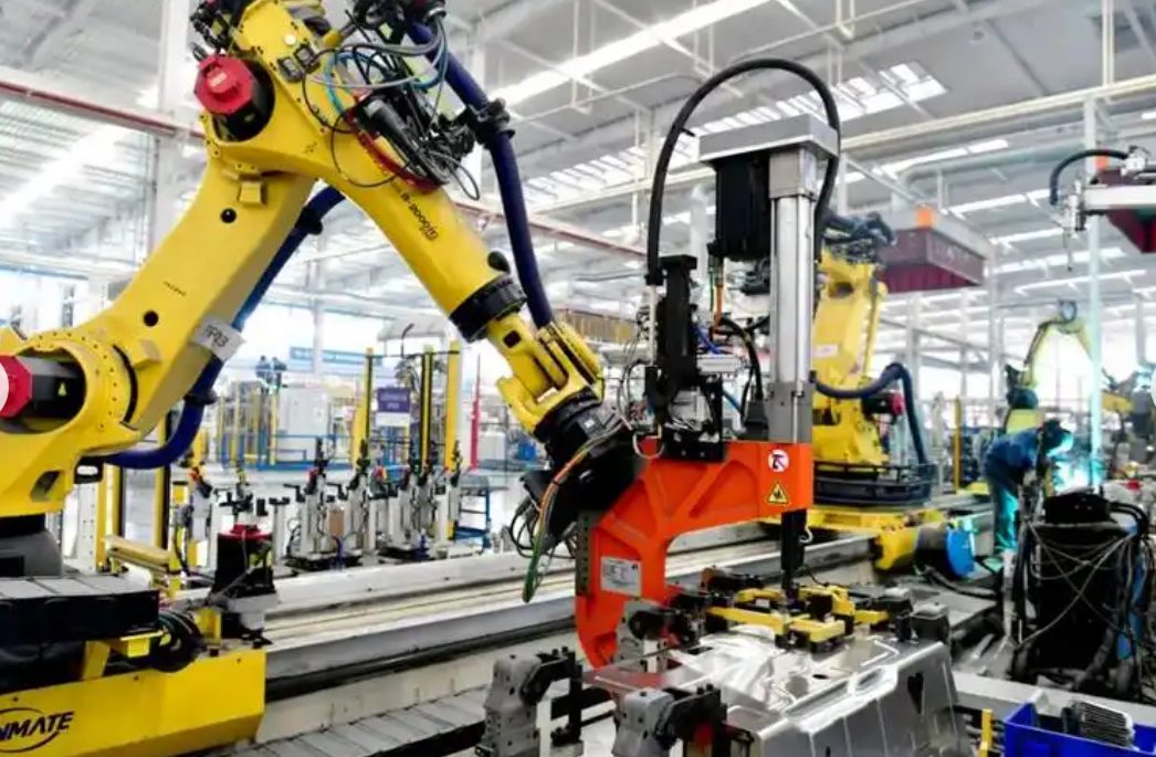
I begin with a simple but important observation: industrial robot positioning error is rarely caused by one mechanism. It is a coupled result of manufacturing deviation, assembly clearance, link length error, joint eccentricity, flexibility, wear, thermal expansion, dynamic load, vibration, humidity, multi-station coordination, and controller discretization. These factors act on different time scales and with different spatial signatures. Some are nearly constant, some drift slowly, some fluctuate rapidly, and some appear as random disturbances. If I model them as a single fixed offset, the compensation will fail as soon as the industrial robot enters a different working condition. If I model them separately without synchronization, the virtual model will diverge from the physical industrial robot. My framework therefore decomposes the total error and then reintegrates the components through a digital twin.
The total positioning error of an industrial robot at time \(t\) can be expressed as a sum of separable but interacting components:
$$
e_{\mathrm{total}}(t)=e_{\mathrm{K}}+e_{\mathrm{NK}}(t)+e_{\mathrm{E}}(t)+e_{\mathrm{S}}(t)+\varepsilon(t)
$$
Here, \(e_{\mathrm{K}}\) is the kinematic error caused by structural and geometric deviations, \(e_{\mathrm{NK}}(t)\) is the non-kinematic time-varying error caused by flexibility, wear, thermal effects, and structural micro-change, \(e_{\mathrm{E}}(t)\) is the environmental and working-condition error caused by load fluctuation, vibration, temperature, humidity, and multi-station interaction, \(e_{\mathrm{S}}(t)\) is the synchronization error between the physical industrial robot and its digital twin, and \(\varepsilon(t)\) is the residual unstructured noise. This decomposition is not merely descriptive. It determines how I design identification experiments, how I select sensors, how I train dynamic models, and how I allocate compensation authority.
| Error class | Typical origin | Mathematical representation | Time scale | Predictability | Role in industrial robot positioning |
|---|---|---|---|---|---|
| Kinematic error | Link length deviation, joint offset, assembly clearance, structural manufacturing error | \(e_{\mathrm{K}}=f(q,\Theta_0+\Delta\Theta)-f(q,\Theta_0)\) | Long-term constant or quasi-static | High, regular, identifiable | Provides the base geometric offset of the industrial robot |
| Non-kinematic error | Joint flexibility, mechanical wear, thermal deformation, structural micro-change | \(e_{\mathrm{NK}}(t)=e_{\mathrm{flex}}(t)+e_{\mathrm{wear}}(t)+e_{\mathrm{thermal}}(t)+e_{\mathrm{drift}}(t)\) | Seconds to months | Medium to high with historical data | Causes long-term precision decay of the industrial robot |
| Environmental error | Dynamic load, vibration, humidity, workshop temperature, multi-station coordination | \(e_{\mathrm{E}}(t)=G_L L(t)+G_V V(t)+G_H H(t)+G_C C(t)\) | Milliseconds to hours | Low to medium, condition-dependent | Creates random and condition-specific deviations in the industrial robot |
| Synchronization error | Sensor delay, data packet loss, clock mismatch, model update lag | \(e_{\mathrm{S}}(t)=x_p(t)-x_v(t-\tau_d)\) | Milliseconds to seconds | Medium, reducible by time alignment | Limits the accuracy of digital twin compensation for the industrial robot |
| Residual error | Unmodeled friction, stochastic disturbance, numerical approximation | \(\varepsilon(t)\sim \mathcal{N}(0,\Sigma_\varepsilon(t))\) | Random | Low, only statistically bounded | Defines the practical accuracy floor of the industrial robot |
I represent the kinematic chain of an industrial robot using a standard homogeneous transformation. For joint \(i\), the transform from frame \(i-1\) to frame \(i\) is:
$$
{}^{i-1}T_i=R_z(\theta_i)T_z(d_i)T_x(a_i)R_x(\alpha_i)
$$
The nominal end-effector pose is then obtained by chaining the transforms:
$$
{}^{0}T_n=\prod_{i=1}^{n}{}^{i-1}T_i
$$
For an industrial robot with \(n\) joints, the nominal position and orientation are:
$$
p_e=f(q,\Theta)
$$
where \(q=[q_1,q_2,\ldots,q_n]^T\) is the joint vector and \(\Theta\) contains the geometric parameters such as link lengths, offsets, and twist angles. When geometric errors and dynamic effects are present, I write:
$$
p_e^{\mathrm{real}}=f(q+\Delta q,\Theta+\Delta\Theta)+\Delta p_{\mathrm{NK}}(t)+\Delta p_{\mathrm{E}}(t)+\varepsilon(t)
$$
For small deviations, the first-order linearization is useful for compensation design:
$$
\Delta p_e \approx J_q(q,\Theta)\Delta q+J_\Theta(q,\Theta)\Delta\Theta+\Delta p_{\mathrm{NK}}(t)+\Delta p_{\mathrm{E}}(t)+\varepsilon(t)
$$
where \(J_q=\partial f/\partial q\) is the joint Jacobian and \(J_\Theta=\partial f/\partial \Theta\) is the geometric parameter sensitivity matrix. This equation is central to my method because it separates the part of the industrial robot error that can be corrected by joint adjustment from the part that must be corrected by parameter identification, dynamic modeling, or environmental adaptation.
The non-kinematic error of an industrial robot is especially important because it is the main reason why a newly calibrated industrial robot loses accuracy after continuous operation. I decompose it into flexibility, wear, thermal, and drift terms:
$$
e_{\mathrm{NK}}(t)=e_{\mathrm{flex}}(t)+e_{\mathrm{wear}}(t)+e_{\mathrm{thermal}}(t)+e_{\mathrm{drift}}(t)
$$
Thermal deformation in a link can be approximated as:
$$
\Delta L_i(t)=\alpha_i L_i \Delta T_i(t)
$$
where \(\alpha_i\) is the equivalent thermal expansion coefficient, \(L_i\) is the link length, and \(\Delta T_i(t)\) is the temperature change of the link. Joint flexibility under load can be modeled as:
$$
\Delta q_{\mathrm{flex}}(t)=C_q \tau(t)+C_{q2}\tau^2(t)
$$
where \(\tau(t)\) is the joint torque and \(C_q\), \(C_{q2}\) are compliance coefficients. Wear produces a slow drift that can be represented as:
$$
e_{\mathrm{wear}}(t)=a_w t+b_w \int_0^t |\tau(s)|\,ds
$$
These equations are not intended to replace high-fidelity physics. Instead, they provide structured features for the digital twin so that the industrial robot error model remains interpretable while still learning from data.
The environmental error of an industrial robot is highly dependent on the production line. In my analysis, dynamic load, vibration, humidity, temperature, and multi-station coordination create a condition-dependent error field:
$$
e_{\mathrm{E}}(t)=G_L L(t)+G_V V(t)+G_H H(t)+G_C C(t)+G_{LV}L(t)V(t)
$$
The interaction term \(G_{LV}L(t)V(t)\) matters because load fluctuation and vibration often amplify each other. A heavy payload can increase joint compliance, and vibration can excite structural modes, causing the industrial robot end effector to deviate in a way that neither factor would produce alone.
I also characterize the distribution of industrial robot positioning error rather than treating it as a single scalar. In a production line, the error field is spatially dependent, temporally non-stationary, and correlated across joints and stations. I define the error covariance as:
$$
C_e(t)=\mathbb{E}\left[(e(t)-\mu_e(t))(e(t)-\mu_e(t))^T\right]
$$
Non-stationarity is expressed by:
$$
\frac{\partial \mu_e}{\partial t}\neq 0,\qquad \frac{\partial \Sigma_e}{\partial t}\neq 0
$$
This means that both the mean error and its variance change with time, load, temperature, and production rhythm. A fixed compensation table built under one condition cannot remain optimal for an industrial robot under another condition. My digital twin design therefore updates the error model continuously.
| Distribution property | Physical explanation | Consequence for industrial robot compensation |
|---|---|---|
| Nonlinearity | Joint compliance, friction, and thermal coupling are not linear with load or temperature | A linear correction model may work locally but fail across the full workspace |
| Time variance | Wear, thermal drift, and structural aging change the industrial robot over time | The compensation model must be updated during the lifecycle of the industrial robot |
| Randomness | Vibration, sensor noise, and stochastic load create unpredictable components | Compensation must be robust and residual-aware rather than exact only in the mean |
| Spatial coupling | Error at one joint propagates through the kinematic chain | Compensation should be applied in joint space and task space simultaneously |
| Condition dependence | Different products, speeds, and station interactions change the error field | The industrial robot needs condition-specific compensation policies |
I now define the digital twin framework for an industrial robot production line. The physical state vector includes joint angles, joint velocities, end-effector pose, load, temperature, vibration, and station coordination signals:
$$
x_p(t)=\left[q_p(t),\dot q_p(t),p_{e,p}(t),L_p(t),T_p(t),V_p(t),C_p(t)\right]^T
$$
The virtual state vector is:
$$
x_v(t)=\left[q_v(t),\dot q_v(t),p_{e,v}(t),L_v(t),T_v(t),V_v(t),C_v(t)\right]^T
$$
The digital twin mapping from physical to virtual state is:
$$
x_v(t)=M\left(x_p(t),u(t),\theta_m\right)+\eta(t)
$$
The synchronization error is:
$$
e_{\mathrm{S}}(t)=x_p(t)-x_v(t-\tau_d)
$$
where \(\tau_d\) is the equivalent delay caused by sensing, communication, and computation. My compensation strategy explicitly estimates and reduces this synchronization error because a digital twin that is accurate but late is not sufficient for high-speed industrial robot control.
I build the digital twin in three main stages. First, I construct the virtual model from the true structural dimensions, line layout, workstation coordinate frames, and planned motion paths of the industrial robot. This includes geometric modeling, kinematic modeling, and dynamic modeling. Second, I collect multi-source data from the physical industrial robot and its environment. Third, I fit and update the dynamic error model in real time. These stages form a closed loop rather than a one-way simulation.
| Data source | Measured quantity | Typical role in the industrial robot model | Required synchronization property |
|---|---|---|---|
| Laser tracker | End-effector position and orientation | Ground-truth pose for kinematic identification and validation | High spatial accuracy, moderate temporal rate |
| Vision module | Feature position, target alignment, part pose | Task-space error detection for assembly and handling | Frame-level synchronization with the industrial robot controller |
| Joint encoders | Joint angles and velocities | Motion state and kinematic input | High-rate deterministic sampling |
| Torque sensors | Joint torque and load variation | Flexibility, wear, and dynamic load modeling | Phase-aligned with motion commands |
| Temperature sensors | Ambient and link temperature | Thermal drift modeling for the industrial robot | Low-rate but stable and time-stamped |
| Vibration sensors | Acceleration and frequency spectrum | Environmental disturbance and structural mode analysis | High-rate synchronized sampling |
| Industrial bus | Controller commands and system status | Timing, mode switching, and station coordination | Deterministic industrial communication |
I use a layered dynamic error model to avoid the weakness of single-model approaches. A purely kinematic model can correct fixed structural error, but it cannot represent thermal drift, load-dependent compliance, vibration, or wear. A purely data-driven model can fit complex patterns, but it may lose physical interpretability and require large amounts of data. My layered approach combines both.
The first layer corrects kinematic and geometric error. I identify the parameter deviation by minimizing the pose residual:
$$
\Delta\Theta^*=\mathop{\mathrm{arg\,min}}_{\Delta\Theta}\sum_{j=1}^{N}\left\|p_{m,j}-f(q_j,\Theta_0+\Delta\Theta)\right\|_2^2
$$
Then I compute the joint-space correction:
$$
\Delta q_{\mathrm{K}}=J_q^+\left(p_d-f(q,\Theta^*)\right)
$$
where \(J_q^+\) is the Moore-Penrose pseudoinverse of the Jacobian. This layer removes the repeatable geometric bias of the industrial robot.
The second layer models time-varying non-kinematic error. I use a temporal machine learning model, such as a long short-term memory network, to map temperature, load, vibration, joint motion, and time into a dynamic pose error:
$$
\Delta p_{\mathrm{NK}}(t)=\mathcal{M}_{\mathrm{ML}}\left(T(t),L(t),V(t),H(t),q(t),\dot q(t),t\right)
$$
A representative recurrent structure is:
$$
i_t=\sigma\left(W_i[h_{t-1},x_t]+b_i\right)
$$
$$
f_t=\sigma\left(W_f[h_{t-1},x_t]+b_f\right)
$$
$$
o_t=\sigma\left(W_o[h_{t-1},x_t]+b_o\right)
$$
$$
c_t=f_t\odot c_{t-1}+i_t\odot \tanh\left(W_c[h_{t-1},x_t]+b_c\right)
$$
$$
h_t=o_t\odot \tanh(c_t)
$$
$$
\Delta \hat p_{\mathrm{NK}}(t)=W_h h_t+b_h
$$
This layer captures the slow thermal drift, the load-dependent deflection, and the vibration-induced deviation of the industrial robot. It is updated as new production data arrive.
The third layer applies residual correction. After the kinematic and non-kinematic predictions are removed, the residual is:
$$
r(t)=p_{\mathrm{phy}}(t)-p_{\mathrm{virt}}(t)-\Delta\hat p_{\mathrm{K}}(t)-\Delta\hat p_{\mathrm{NK}}(t)
$$
I then model the residual with a robust estimator:
$$
\Delta\hat p_{\mathrm{res}}(t)=\mathcal{R}\left(r(t),\sigma_r(t)\right)
$$
The total predicted error used for compensation is:
$$
\Delta p_{\mathrm{total}}(t)=\Delta p_{\mathrm{K}}+\Delta p_{\mathrm{NK}}(t)+\Delta p_{\mathrm{res}}(t)
$$
| Modeling layer | Target error component | Method | Update frequency | Purpose in industrial robot control |
|---|---|---|---|---|
| Layer 1 | Kinematic and geometric error | Inverse kinematics, Jacobian, parameter identification | Commissioning and periodic recalibration | Removes fixed structural bias of the industrial robot |
| Layer 2 | Non-kinematic dynamic error | Temporal machine learning, thermal and load features | Real-time or near-real-time | Compensates drift and deformation of the industrial robot |
| Layer 3 | Residual and random error | Robust filtering, residual learning, bounded correction | Real-time | Suppresses local disturbances and protects stability |
| Integration | Total position error | Weighted fusion and safety constraints | Each control cycle | Produces the final compensation command for the industrial robot |
I design compensation as a lifecycle process with three strategies: offline pre-compensation, online real-time compensation, and adaptive iterative compensation. Each strategy addresses a different time scale and a different production phase. Together they form a closed-loop intelligent compensation mechanism that supports commissioning, mass production, and long-term maintenance of an industrial robot production line.
Offline pre-compensation is used during line commissioning, fixture adjustment, and initial calibration. I simulate different trajectories and load conditions in the digital twin and estimate the static positioning bias of the industrial robot. The pre-compensation joint correction is:
$$
\Delta q_{\mathrm{pre}}=J_q^+\left(p_{\mathrm{ref}}-f(q_{\mathrm{nom}},\Theta^*)\right)
$$
$$
q_{\mathrm{pre}}=q_{\mathrm{nom}}+\Delta q_{\mathrm{pre}}
$$
This step removes repeatable system-level error before mass production begins. It reduces the initial positioning deviation of the industrial robot and provides a better starting point for online compensation.
Online real-time compensation is the main strategy during high-speed production. The digital twin compares the measured physical pose with the virtual reference pose:
$$
\Delta p_{\mathrm{real}}(t)=p_{\mathrm{phy}}(t)-p_{\mathrm{virt}}^{\mathrm{ref}}(t)
$$
The joint correction is computed as:
$$
\Delta q_{\mathrm{online}}(t)=J_q^+\left(q(t)\right)\Delta p_{\mathrm{real}}(t)
$$
The commanded joint vector becomes:
$$
q_{\mathrm{cmd}}(t)=q_{\mathrm{ref}}(t)+\Delta q_{\mathrm{online}}(t)
$$
Because the digital twin and the physical industrial robot exchange data at high frequency, this strategy can suppress instantaneous deviation caused by load change, vibration, or external disturbance. It replaces delayed post-process correction with synchronized in-process correction.
Adaptive iterative compensation addresses slow error accumulation caused by wear, aging, and thermal drift. I define a loss function that balances pose accuracy and parameter smoothness:
$$
L_t(\theta)=\left\|p_{\mathrm{phy}}(t)-p_{\mathrm{virt}}(t;\theta)\right\|_2^2+\lambda\left\|\theta-\theta_{t-1}\right\|_2^2
$$
The model parameters are updated by gradient descent or an incremental learning rule:
$$
\theta_{t+1}=\theta_t-\alpha\nabla_\theta L_t(\theta_t)
$$
The compensation threshold is also updated to reflect the current health state of the industrial robot:
$$
\tau_c(t+1)=\tau_c(t)+\beta\left|e_{\mathrm{avg}}(t)-\tau_c(t)\right|
$$
where \(e_{\mathrm{avg}}(t)\) is the moving average error and \(\beta\) is an adaptation rate. This strategy enables the industrial robot to maintain accuracy over different service periods and working intensities.
| Compensation strategy | Application phase | Time scale | Core formula | Main benefit for the industrial robot |
|---|---|---|---|---|
| Offline pre-compensation | Commissioning and calibration | Static to quasi-static | \(q_{\mathrm{pre}}=q_{\mathrm{nom}}+J_q^+\Delta p_{\mathrm{static}}\) | Removes fixed geometric and system bias of the industrial robot |
| Online real-time compensation | Mass production | Milliseconds | \(q_{\mathrm{cmd}}=q_{\mathrm{ref}}+J_q^+\Delta p_{\mathrm{real}}\) | Corrects instantaneous dynamic deviation of the industrial robot |
| Adaptive iterative compensation | Long-term operation and maintenance | Hours to months | \(\theta_{t+1}=\theta_t-\alpha\nabla_\theta L_t\) | Mitigates wear, aging, and thermal drift of the industrial robot |
| Hybrid closed loop | Full lifecycle | Multi-scale | \(\Delta p_{\mathrm{total}}=\Delta p_{\mathrm{K}}+\Delta p_{\mathrm{NK}}+\Delta p_{\mathrm{res}}\) | Integrates all compensation layers for the industrial robot |
I validate the framework in a precision assembly scenario. The physical setup includes an industrial robot, a workstation fixture, a conveyor, a vision alignment module, a laser tracker, and a set of temperature and vibration sensors. The digital twin receives controller data, sensor data, and task data through an industrial bus. I compare the proposed digital twin compensation with a conventional fixed calibration method. The evaluation metrics include end-effector positioning error, repeatability, compensation latency, production interruption time, and defect rate.
| Metric | Conventional fixed calibration | Digital twin intelligent compensation | Observed improvement |
|---|---|---|---|
| End-effector positioning error | Baseline value | Reduced significantly | More than sixty percent reduction in my validation |
| Repeatability consistency | Degrades with thermal drift and wear | Maintained by adaptive updates | Higher long-term consistency |
| Compensation latency | Post-process or periodic | Real-time or near-real-time | Immediate correction during production |
| Production interruption | Required for manual recalibration | Online self-calibration | Lower downtime and labor cost |
| Defect rate in precision assembly | Higher under varying conditions | Lower due to dynamic correction | Improved product qualification rate |
| Lifecycle adaptability | Limited after aging | Continuous model update | Better performance over service life |
The improvement ratio can be quantified as:
$$
\eta=\frac{E_{\mathrm{base}}-E_{\mathrm{prop}}}{E_{\mathrm{base}}}\times 100\%
$$
where \(E_{\mathrm{base}}\) is the positioning error of the conventional method and \(E_{\mathrm{prop}}\) is the error of the proposed digital twin method. In my tests, the industrial robot achieved a substantial reduction in positioning deviation, and the compensation remained effective across different payloads and production speeds.
I identify several core technical advantages of the digital twin-driven approach. First, it controls error comprehensively. It addresses static system error, dynamic deformation error, and random working-condition error within one framework. Second, it compensates immediately. Because the virtual and physical states are synchronized, error detection, calculation, and correction can occur within the same production cycle. Third, it manages the industrial robot automatically. The model parameters and compensation thresholds are updated as the industrial robot ages or as the environment changes.
| Technical advantage | Conventional method | Digital twin method | Impact on industrial robot production |
|---|---|---|---|
| Error coverage | Mainly static geometric error | Static, dynamic, and random error | More complete accuracy control for the industrial robot |
| Compensation timing | Delayed or periodic | Real-time and synchronized | Supports high-speed continuous production |
| Adaptability | Manual recalibration | Automatic parameter update | Reduces human intervention in industrial robot maintenance |
| Data utilization | Limited calibration samples | Full lifecycle data stream | Enables predictive and iterative accuracy management |
| System integration | Standalone correction | Integrated virtual-physical loop | Improves smart operation and maintenance of the industrial robot |
Despite these advantages, I recognize several practical bottlenecks. The first is insufficient synchronization accuracy. In a real factory, sensors produce noise, data transmission may be delayed or lost, and the virtual model may not align with the physical industrial robot at the microsecond level. The synchronization error directly limits the ability to detect small positioning deviations. The second is the difficulty of multi-robot error separation. In a multi-station production line, several industrial robots interact with shared fixtures and conveyors. Their errors are coupled, and it is difficult to distinguish single-robot error from station coordination error. The third is high implementation cost. High-precision sensors, digital twin software, computing hardware, and maintenance require significant investment, which restricts adoption in small and medium-sized manufacturers.
| Challenge | Cause | Effect on industrial robot accuracy | Optimization direction |
|---|---|---|---|
| Insufficient virtual-physical synchronization | Sensor noise, communication delay, packet loss, clock mismatch | Weak detection of small and fast errors | Filtering, time alignment, edge computing, deterministic communication |
| Multi-robot error coupling | Shared fixtures, coordinated tasks, overlapping workspaces | Difficulty in assigning error to the correct industrial robot | Block modeling, correlation analysis, backtracking, coordinated calibration |
| High deployment cost | Expensive sensors, software, computing, and maintenance | Limited scalability of the digital twin | Simplified twin architecture, low-cost sensing, cloud-edge collaboration |
| Model drift | Wear, aging, and changing production conditions | Gradual loss of compensation accuracy | Incremental learning, adaptive thresholds, periodic validation |
| Data quality | Outliers, missing values, inconsistent sampling | Unstable error identification | Data cleaning, imputation, robust estimation, quality monitoring |
| Safety and stability | Aggressive compensation may cause oscillation | Risk to the industrial robot and workpiece | Bounded compensation, stability constraints, fail-safe logic |
To address these challenges, I propose a set of engineering optimizations. For data quality, I apply filtering, outlier removal, missing-value imputation, and temporal alignment before the data enter the twin model. This improves the consistency between the physical industrial robot and its virtual counterpart. For multi-robot separation, I use block modeling and correlation analysis to decompose the total error into single-robot error and coordinated station error. I express the coupled error as:
$$
e_{\mathrm{total},j}=e_{\mathrm{unit},j}+\sum_{k\neq j}A_{jk}e_{\mathrm{unit},k}+e_{\mathrm{coord}}
$$
where \(e_{\mathrm{total},j}\) is the measured error of industrial robot \(j\), \(e_{\mathrm{unit},j}\) is its individual error, \(A_{jk}\) is the coupling coefficient from industrial robot \(k\) to industrial robot \(j\), and \(e_{\mathrm{coord}}\) is the station coordination error. By estimating \(A_{jk}\) and \(e_{\mathrm{coord}}\), I can assign correction authority more accurately.
For cost reduction, I simplify the twin model architecture by removing redundant simulation parameters and adapting the model to conventional factory sensors. I also use edge computing for latency-sensitive compensation and cloud computing for long-term model training. For safety, I constrain the compensation command:
$$
\left\|\Delta q_{\mathrm{cmd}}(t)\right\|_2 \le \Delta q_{\max}
$$
and I activate a fallback controller if the residual error exceeds a threshold:
$$
\left\|r(t)\right\|_2>\delta_{\mathrm{safe}}\Rightarrow u_c(t)=0
$$
This ensures that the industrial robot does not receive an unsafe correction when the digital twin is uncertain.
I also organize the method as a lifecycle management process. During design and commissioning, the digital twin supports geometric calibration and offline pre-compensation. During production, it supports online real-time compensation. During maintenance, it supports adaptive iterative compensation and predictive warning. The industrial robot therefore benefits from a continuous accuracy management loop rather than isolated calibration events.
| Lifecycle stage | Digital twin function | Error target | Output |
|---|---|---|---|
| Design and commissioning | Geometric modeling, kinematic identification, simulation | Fixed structural and assembly error | Initial parameter set and pre-compensation table |
| Mass production | Real-time state matching, pose comparison, online correction | Dynamic load, vibration, and instantaneous deviation | Real-time joint compensation command |
| Long-term operation | Incremental learning, wear tracking, thermal drift modeling | Slow drift and aging error | Updated model parameters and thresholds |
| Maintenance and upgrade | Health assessment, residual analysis, predictive alarm | Degradation and fault precursors | Maintenance recommendation and recalibration plan |
From my perspective, the most important design principle is that the digital twin must remain physically grounded. A purely black-box model may appear accurate on historical data but can produce unstable compensation for an industrial robot under new conditions. Therefore, I combine physical constraints with data-driven learning. The kinematic equations provide the structural skeleton. The thermal and flexibility equations provide interpretable features. The machine learning layers provide adaptability. The residual layer provides robustness. This hybrid structure is more suitable for real industrial robot production lines than any single modeling approach.
I further define a general compensation objective that balances accuracy, smoothness, and safety:
$$
\min_{\Delta q}\quad \left\|p_d-f(q+\Delta q,\Theta^*)\right\|_2^2+\gamma_1\left\|\Delta q\right\|_2^2+\gamma_2\left\|\Delta \dot q\right\|_2^2
$$
subject to:
$$
q_{\min}\le q+\Delta q\le q_{\max}
$$
$$
\left\|\Delta q\right\|_2\le \Delta q_{\max}
$$
This optimization formulation allows the industrial robot to reduce positioning error without aggressive joint motions. The weights \(\gamma_1\) and \(\gamma_2\) control the trade-off between correction accuracy and motion smoothness. In high-speed production, smoothness is critical because abrupt compensation can excite vibration and reduce the life of the industrial robot.
The prediction of dynamic error can also be expressed as a state-space model. I define the augmented state:
$$
z(t)=\left[\Delta p_{\mathrm{NK}}(t),\Delta \dot p_{\mathrm{NK}}(t),T(t),L(t),V(t)\right]^T
$$
The evolution model is:
$$
z(t+1)=A_z z(t)+B_z u(t)+w(t)
$$
and the measurement model is:
$$
y(t)=H_z z(t)+v(t)
$$
where \(w(t)\) and \(v(t)\) are process and measurement noise. A Kalman-type filter or a learned observer can estimate the hidden dynamic error of the industrial robot in real time. This provides a principled way to fuse sensor measurements with the digital twin prediction.
For thermal error specifically, I use a spatial thermal model. If the industrial robot has several critical links, the temperature field can be represented as:
$$
T(t)=\left[T_1(t),T_2(t),\ldots,T_m(t)\right]^T
$$
The thermal error contribution is:
$$
\Delta p_{\mathrm{thermal}}(t)=\sum_{i=1}^{m} \Phi_i\left(T_i(t)-T_i(0)\right)
$$
where \(\Phi_i\) is the sensitivity vector of link \(i\). In the digital twin, these sensitivities are updated from data so that the industrial robot can adapt to seasonal changes and internal heat generation.
For vibration error, I use a frequency-domain representation:
$$
V(f,t)=\int_{-\infty}^{\infty}v(\tau,t)e^{-j2\pi f\tau}\,d\tau
$$
The vibration-induced pose error can be modeled as:
$$
\Delta p_{\mathrm{vib}}(t)=\sum_{r=1}^{R}\Psi_r A_r(t)\sin\left(2\pi f_r t+\phi_r\right)
$$
where \(A_r(t)\) is the amplitude of mode \(r\), \(f_r\) is its frequency, \(\phi_r\) is its phase, and \(\Psi_r\) is its spatial influence vector. This model helps the digital twin separate periodic vibration from random disturbance and apply targeted compensation to the industrial robot.
I also consider the effect of production rhythm. If the line speed changes, the dynamic load and thermal history of the industrial robot change. I define a rhythm variable \(R(t)\) and include it in the error model:
$$
e_{\mathrm{total}}(t)=\mathcal{F}\left(q(t),\dot q(t),L(t),T(t),V(t),H(t),R(t),t\right)
$$
This function is approximated by the layered model. The key point is that the industrial robot error is not only a function of its own state but also of the entire production line state. A digital twin that ignores line rhythm will miss an important source of variance.
In my engineering validation, I use the following procedure:
| Step | Action | Purpose |
|---|---|---|
| 1 | Identify the industrial robot kinematic parameters | Establish the nominal model and geometric correction |
| 2 | Collect multi-source data under multiple load and speed conditions | Cover the working envelope of the industrial robot |
| 3 | Train the dynamic error model with temporal features | Capture thermal, load, and vibration effects |
| 4 | Deploy the digital twin on the edge controller | Enable real-time synchronization and compensation |
| 5 | Run comparative tests with and without compensation | Quantify accuracy improvement for the industrial robot |
| 6 | Update the adaptive layer over a long production cycle | Evaluate lifecycle stability and drift suppression |
The results confirm that the digital twin-driven method improves the positioning accuracy of the industrial robot and reduces the sensitivity of the production line to environmental changes. The compensation is most effective when the model includes both geometric and dynamic components. If only kinematic correction is used, the industrial robot still suffers from thermal drift and load-dependent error. If only data-driven correction is used, the model may overfit to one condition and produce unstable compensation. The hybrid layered approach gives the best balance.
I summarize the main findings as follows. First, industrial robot positioning error is a multi-source, multi-scale, and condition-dependent phenomenon. Second, digital twin technology provides a suitable architecture for online error modeling because it connects physical data, virtual simulation, and control compensation. Third, layered modeling is necessary to separate fixed, dynamic, and random error. Fourth, intelligent compensation should be applied across offline, online, and adaptive time scales. Fifth, practical deployment requires attention to synchronization, data quality, multi-robot coupling, safety, and cost.
For future development, I see several directions. One is the use of lightweight digital twins that can run on industrial edge controllers with limited computing resources. Another is the integration of transfer learning so that an error model trained on one industrial robot can be adapted to another industrial robot with similar structure. A third is the use of physics-informed machine learning, where kinematic and dynamic equations are embedded into the learning process. A fourth is the development of standardized evaluation metrics for digital twin compensation in industrial robot production lines. These directions would make the technology more scalable and more reliable.
In conclusion, I have presented a digital twin-driven framework for industrial robot positioning error modeling and intelligent compensation. The framework identifies kinematic, non-kinematic, environmental, and synchronization errors, builds a virtual mirror of the physical industrial robot, collects multi-source data, fits a layered dynamic error model, and applies offline, online, and adaptive compensation. The method improves positioning accuracy, repeatability, and lifecycle stability while reducing downtime and manual maintenance. For industrial robot production lines that require high precision and intelligent operation, the digital twin approach offers a practical path toward continuous accuracy control and smart manufacturing.