
The field of legged robotics represents a significant frontier in creating machines capable of navigating complex, unstructured environments. Unlike their wheeled counterparts, legged robots possess the unique ability to traverse terrains with discrete and uneven footholds, such as rubble, stairs, or natural landscapes. This capability makes them invaluable for applications ranging from search and rescue and hazardous environment exploration to advanced military logistics and personal entertainment. Within this domain, quadrupedal robots strike a critical balance between stability, mechanical complexity, and control sophistication. They offer superior payload capacity and static stability compared to bipeds, while being inherently less complex than hexapod or octopod platforms. A core challenge in realizing the potential of a robot dog is the generation of stable, efficient, and high-speed dynamic walking gaits. This article delves into the detailed gait planning and simulation for a quadruped robot dog, focusing on the dynamic trot gait as a pathway to rapid locomotion.
Gait, in the context of a legged robot dog, refers to the coordinated, rhythmic sequence of leg movements that result in net displacement of the body. The fundamental challenge lies in ensuring continuous stability—keeping the robot’s center of gravity (CoG) within the polygon of support formed by the legs in contact with the ground—while executing these movements. Gaits are typically analyzed using gait diagrams, which plot the state (stance or swing) of each leg over time. Key parameters defining a gait include the stride length $\lambda$, the cycle time $T$, and most importantly, the duty factor $\beta$.
The duty factor $\beta_i$ for leg $i$ is defined as the fraction of the total gait cycle period that the leg remains in the stance phase (supporting the body):
$$
\beta_i = \frac{T_{stance,i}}{T_{cycle}}
$$
For a quadruped, the value of $\beta$ determines the number of legs in support at any given instant and thus categorizes the gait:
| Duty Factor ($\beta$) | Legs in Support | Gait Characteristic | Typical Gait Name |
|---|---|---|---|
| $\beta > 0.5$ | 3 or 4 | Always at least 3 legs grounded. High stability, lower speed. | Walk (e.g., Crawl) |
| $\beta = 0.5$ | 2 | Exactly 2 legs grounded. Dynamic stability required, higher speed. | Trot |
| $\beta < 0.5$ | 1 or 0 | Flight phases present. Requires advanced control and mechanical compliance. | Gallop, Bound |
This study focuses on the trot gait ($\beta=0.5$), a dynamic and efficient gait where diagonal leg pairs move in synchrony. This gait is a primary target for achieving running speeds in a quadruped robot dog.
Mechanical Architecture and Kinematic Modeling of the Robot Dog
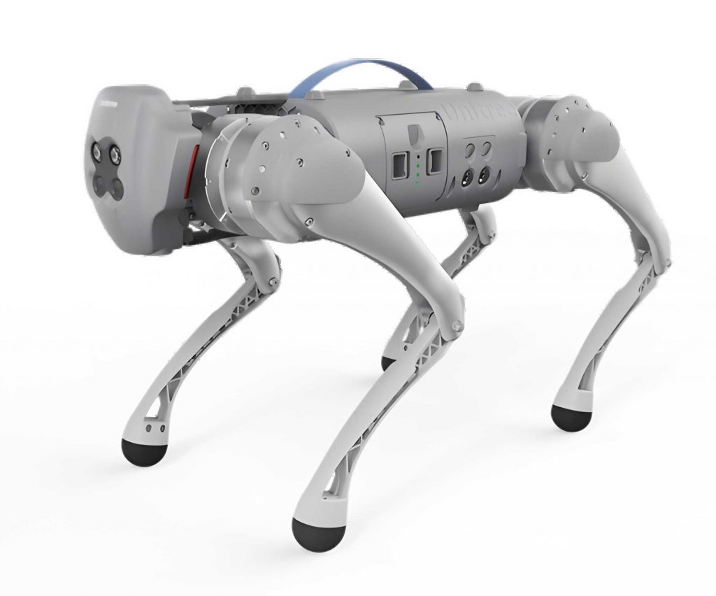
The mechanical design of the robot dog is fundamental to its mobility. The leg architecture typically consists of multiple serially connected links actuated by rotary joints. For a mammalian-inspired robot dog, each leg often features three primary active degrees of freedom (DoF):
- Hip Abduction/Adduction: Swing the leg laterally (in/out).
- Hip Flexion/Extension: Swing the leg forward/backward.
- Knee Flexion/Extension: Extend or retract the lower leg.
An additional passive or compliant ankle joint may be included to improve ground contact and force distribution. For simplicity in basic gait analysis, the lateral motion (abduction/adduction) is often neglected for straight-line walking, reducing the model to a 2-DoF planar manipulator per leg in the sagittal plane: a hip pitch joint and a knee pitch joint.
A simplified kinematic model for one leg of the robot dog in the sagittal plane can be defined. Let the robot’s body frame be the world frame at the hip joint. The leg has an upper link (thigh) of length $L_1$ and a lower link (shank) of length $L_2$. The hip joint angle $\theta_1$ is measured from the body horizontal, and the knee joint angle $\theta_2$ is measured relative to the thigh. The position of the foot (end-effector) $(p_x, p_z)$ relative to the hip is given by the forward kinematics:
$$
\begin{aligned}
p_x &= L_1 \cos(\theta_1) + L_2 \cos(\theta_1 + \theta_2) \\
p_z &= L_1 \sin(\theta_1) + L_2 \sin(\theta_1 + \theta_2)
\end{aligned}
$$
The inverse kinematics, crucial for placing the foot at desired positions, can be solved geometrically. Given a desired foot position $(p_x, p_z)$, the distance from the hip to the foot is $D = \sqrt{p_x^2 + p_z^2}$. Using the law of cosines, the knee angle $\theta_2$ is:
$$
\theta_2 = \pi – \arccos\left( \frac{L_1^2 + L_2^2 – D^2}{2 L_1 L_2} \right)
$$
The hip angle $\theta_1$ is then:
$$
\theta_1 = \atan2(p_z, p_x) – \atan2\left( L_2 \sin(\theta_2), L_1 + L_2 \cos(\theta_2) \right)
$$
This model forms the basis for planning the trajectory of each foot during swing and stance phases for the robot dog.
Principles and Planning of the Diagonal Trot Gait
The trot is a symmetrical gait where the legs move in diagonal pairs. We define the legs as: Left-Front (LF), Right-Front (RF), Left-Hind (LH), Right-Hind (RH). In a trot, the diagonal pairs (LF-RH) and (RF-LH) are coupled. When one diagonal pair is in the swing phase, the other is in the stance phase, and they switch roles at the midpoint of the cycle. For a robot dog to remain balanced during a trot, its body motion must be actively coordinated with the leg movements, as the support polygon reduces to a line connecting the two stance feet. Stability is achieved through dynamic principles, often involving the control of the body’s pitch and roll, rather than static stability.
The gait cycle $T$ is divided into two main phases of duration $T/2$ each. During the first half-cycle, one diagonal pair (e.g., LF and RH) swings forward while the other pair (RF and LH) pushes the body forward. The roles are reversed in the second half-cycle. The foot trajectory for each leg during its swing phase is typically planned as a smooth curve (e.g., a cycloid or polynomial) that lifts the foot clear of the ground, moves it forward, and places it down with minimal impact. The stance leg follows a prescribed trajectory relative to the moving body to propel it forward.
Let us define a body coordinate system where the $+X$ axis points forward, the $+Z$ axis points upward, and the origin is at the body’s geometric center. The planned motion for one complete trot cycle can be broken down into a sequence for a diagonal pair. For the (RF-LH) pair, the joint angle sequences are planned to create the following body displacement of stride length $\lambda$:
| Phase (Duration $T/4$) | RF Hip $\theta_{RH}$ | RF Knee $\theta_{RK}$ | LH Hip $\theta_{LH}$ | LH Knee $\theta_{LK}$ | Primary Action |
|---|---|---|---|---|---|
| Phase 1: Initial Swing/Stance Transition | $- \alpha$ (Extend) | $+ \delta$ (Flex) | $+ \alpha$ (Flex) | $0$ (Hold) | RH swings back; LH holds for propulsion. |
| Phase 2: Mid-cycle Switch | $+ \alpha$ (Flex) | $- \delta$ (Extend) | $- \alpha$ (Extend) | $0$ (Hold) | RH swings forward to prepare for touch-down; LH continues propulsion. |
| Phase 3: Second Swing/Stance Transition | $+ \alpha$ (Flex) | $0$ (Hold) | $- \alpha$ (Extend) | $+ \delta$ (Flex) | LH swings back; RH now in stance, holds. |
| Phase 4: Return to Initial Configuration | $- \alpha$ (Extend) | $0$ (Hold) | $+ \alpha$ (Flex) | $- \delta$ (Extend) | LH swings forward; RH holds. Body has advanced by $\lambda$. |
The angles $\alpha$ and $\delta$ are determined by the desired stride length $\lambda$ and maximum foot clearance $h_{max}$ via the inverse kinematics equations. The motion of the (LF-RH) diagonal pair is exactly $180^\circ$ (or $T/2$) out of phase with the (RF-LH) pair. This inter-leg coordination is the cornerstone of the trot gait for the robot dog. The body’s forward velocity $v_{body}$ is related to the stride length and cycle time by $v_{body} = \lambda / T$.
Simulation Environment and Dynamic Model
To validate the gait plan without physical prototyping, a dynamic simulation is essential. The simulation builds upon the kinematic model by incorporating masses, inertias, and the forces/torques required to produce the planned motion. A simplified yet effective approach uses a planar model of the robot dog, focusing on the sagittal (X-Z) plane motion during straight-line trotting.
The robot’s body is treated as a single rigid body of mass $M_b$ and moment of inertia $I_b$ about its CoG. Each leg link has mass $m_i$ and inertia $I_i$. The equations of motion are derived using the Lagrangian method or recursive Newton-Euler algorithms. For simulation, the planned joint angle trajectories $\theta_d(t)$ become the desired positions for a low-level joint controller. A common model is a proportional-derivative (PD) controller that generates joint torque $\tau$:
$$
\tau = K_p (\theta_d – \theta) + K_d (\dot{\theta}_d – \dot{\theta})
$$
where $K_p$ and $K_d$ are proportional and derivative gain matrices, and $\theta$ is the actual joint angle.
The ground interaction is modeled using a spring-damper system for the foot in contact. When a foot is in stance, a vertical ground reaction force $F_z$ is generated if the foot penetrates the ground by a depth $z$:
$$
F_z = \begin{cases}
-k z – c \dot{z}, & \text{if } z > 0 \text{ (penetration)} \\
0, & \text{otherwise}
\end{cases}
$$
where $k$ is the ground stiffness and $c$ is the damping coefficient. Friction in the forward direction can be modeled with a Coulomb friction model.
The simulation is implemented in a numerical environment like MATLAB/Simulink or Python with physics engines (e.g., PyBullet, MuJoCo). The process involves:
- Defining the physical parameters (link lengths, masses, inertias) of the robot dog.
- Implementing the trot gait planner to generate the time-series data for desired joint angles $\theta_d(t)$ for all legs over multiple cycles.
- Implementing the joint-level PD controllers.
- Integrating the full system dynamics using a numerical solver (e.g., ODE45).
- Recording and analyzing state variables: body position $(X_b, Z_b)$, orientation, joint angles, joint torques, ground reaction forces, and the Zero-Moment Point (ZMP) or Center of Pressure (CoP).
Simulation Results and Analysis for the Robot Dog Trot
Executing the simulation with the planned trot gait yields critical data on the performance and stability of the robot dog. The following results are typically observed from a well-tuned simulation:
1. Body Trajectory: The body’s CoG exhibits characteristic oscillations.
- Forward (X) Displacement: Shows a steady increase with small periodic fluctuations corresponding to the stride cycle. The average slope gives the forward speed $v_{body}$.
- Vertical (Z) Displacement: The body bounces with a period of $T/2$ (twice per full gait cycle), as each diagonal leg pair’s thrust and the body’s compliance cause it to rise and fall. The amplitude should be bounded and relatively small for energy efficiency.
- Lateral (Y) Displacement: In a perfectly symmetric trot on flat ground, lateral displacement should be minimal. However, initial conditions or asymmetries might cause a small drift, which the controller must correct.
2. Footfall Pattern and Ground Reaction Forces (GRFs): The simulation visually confirms the correct phasing of the diagonal leg pairs. The GRF plots for each foot show two distinct peaks per gait cycle, corresponding to the thrusting phase of each stance leg. The forces should be smoothly distributed to avoid large impacts.
3. Joint Kinematics and Dynamics: The actual joint angles $\theta(t)$ closely track the desired trajectories $\theta_d(t)$, with slight deviations due to dynamic coupling and link inertia. The joint torques $\tau(t)$ provide insight into the actuator requirements. Peak torques occur during the thrust phase of stance and the liftoff phase of swing.
4. Stability Metrics: The trajectory of the Zero-Moment Point (ZMP) is a key stability indicator. For dynamic gaits like the trot, the ZMP does not need to remain strictly within the support polygon (which is a line), but its motion should be controlled and oscillate around the center of the support line. Large, uncontrolled excursions of the ZMP indicate instability.
A summary of quantitative results from a sample simulation might look like this:
| Performance Metric | Simulation Value | Notes |
|---|---|---|
| Gait Cycle Time, $T$ | 1.0 s | Defined by planner |
| Duty Factor, $\beta$ | 0.5 | Trot gait |
| Stride Length, $\lambda$ | 0.25 m | Planned forward displacement per cycle |
| Average Forward Speed, $v_{body}$ | 0.25 m/s | Calculated as $\lambda / T$ |
| Max Body Vertical Oscillation | $\pm 0.005$ m | Acceptably small bounce |
| Peak Hip Joint Torque | 12.5 Nm | Sizing requirement for actuators |
| Peak Knee Joint Torque | 8.2 Nm | Sizing requirement for actuators |
| ZMP Lateral Excursion | $\pm 0.02$ m | Controlled, indicates dynamic stability |
The simulation confirms the viability of the planned trot gait. The robot dog model successfully progresses forward with a stable, periodic motion. The joint torques remain within feasible limits for standard servo or BLDC motors, and the body motion is reasonably smooth. Discrepancies between planned and simulated paths, such as slight body pitching or energy losses, highlight areas for improvement in the control laws or mechanical design, such as adding series elastic actuators (SEAs) for better compliance and energy storage.
Conclusion
This comprehensive analysis demonstrates a methodology for gait planning and simulation of a quadruped robot dog, with a focused application on the dynamic trot gait. By establishing a simplified yet representative kinematic and dynamic model, planning the coordinated diagonal leg movements, and implementing a physics-based simulation, the feasibility and characteristics of the gait can be thoroughly investigated before physical implementation. The simulation results provide critical insights into body trajectories, actuator requirements, and dynamic stability metrics, all of which are essential for the successful development of a agile and robust robot dog. The trot gait, with its duty factor of 0.5, serves as a foundational stepping stone towards even more dynamic and high-speed gaits like the gallop. Future work would involve extending the model to 3D, incorporating more sophisticated whole-body controllers, optimizing gait parameters for energy efficiency, and validating the simulation results on a physical robot dog platform. The iterative cycle of modeling, planning, simulation, and physical testing remains the core paradigm for advancing the capabilities of legged robotic systems.