
As a researcher in mechanical engineering, I have long been fascinated by the intricate dynamics of precision transmission systems, particularly the RV reducer, which is pivotal in industrial robotics due to its high reduction ratio, compact size, and robustness. In this article, I will delve into a critical aspect of RV reducer design: the dynamic load characteristics of needle roller bearings under the influence of position errors. The RV reducer relies on a combination of planetary gears and cycloidal-pin transmissions, where needle roller bearings serve as the turning arm bearings, often without inner or outer rings to save space. These bearings are subjected to complex, fluctuating loads, and their failure can severely compromise the reducer’s reliability and lifespan. My focus here is to explore how machining position errors in the bearing holes of cycloidal gears affect the dynamic contact loads across multiple sets of bearings, leading to uneven load-sharing and potential fatigue issues. Through a comprehensive dynamic model that integrates multi-group needle roller bearings with cycloidal-pin transmissions, I aim to provide insights that can enhance the design and durability of RV reducers.
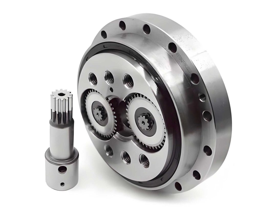
The RV reducer operates under high-stress conditions, where the needle roller bearings facilitate the motion between the crankshafts and cycloidal gears. However, in practical manufacturing, position errors—deviations in the angular and radial placement of bearing holes on cycloidal gears—are inevitable due to machining tolerances. These errors can alter the load distribution among bearings, causing some to bear excessive loads while others are underutilized. This uneven load-sharing not only accelerates wear and tear but also leads to premature failure of the RV reducer. To address this, I have developed a dynamic model that incorporates these position errors, allowing for a detailed analysis of their impact on bearing loads. My approach combines multi-point contact modeling for both the cycloidal-pin meshing and the needle roller bearings, coupled with a systematic representation of position errors. This model enables me to simulate real-world operating conditions and quantify the effects of error magnitudes on load fluctuations and bearing performance.
In the following sections, I will first outline the theoretical foundation of my dynamic model, including the mathematical formulations for contact forces in cycloidal-pin pairs and needle roller bearings. I will then explain how position errors are integrated into the model, followed by the assembly of the overall coupled transmission mechanism dynamics. Subsequently, I will present a case study based on a typical RV80E reducer with three crankshafts, using tables and formulas to summarize parameters and results. Finally, I will discuss the implications of my findings for the design and manufacturing of RV reducers, emphasizing the need for precision control to ensure optimal load distribution and longevity.
My methodology begins with the multi-point contact modeling of the cycloidal-pin transmission. The cycloidal gear profile is derived from standard equations, but for contact analysis, I discretize the profile into points to assess interactions with pin teeth. Let me define the global coordinate system as \( XOY \), with local coordinates for cycloidal gear A as \( A A A x_o y \) and for cycloidal gear B as \( B B B x_o y \). The position vector of a discretized point on the cycloidal gear in the global system is given by:
$$ \mathbf{r}_z^d = \mathbf{r}_z^c + \mathbf{A}_z^c \mathbf{s}_z^c $$
where \( z \) denotes the cycloidal gear (A or B), \( \mathbf{r}_z^c \) is the position vector of the gear’s center, \( \mathbf{s}_z^c \) is the position vector in the local coordinate system, and \( \mathbf{A}_z^c \) is the transformation matrix. For a pin with center at \( \mathbf{r}_j^p \), the relative position vector is:
$$ \mathbf{d}_j^z = \mathbf{r}_j^p – \mathbf{r}_z^d $$
Contact occurs when the magnitude of \( \mathbf{d}_j^z \) is less than the pin radius \( r_r \), i.e., \( \| \mathbf{d}_j^z \| – r_r < 0 \). The contact depth \( \delta_j^z \) is calculated as:
$$ \delta_j^z = \| \mathbf{d}_j^z \| – r_r $$
Within a contact region, multiple points may satisfy this condition; I select the point with maximum depth as the contact point. The normal direction vector \( \mathbf{n}_j^z \) is derived from the relative position vector at this point. The normal contact force \( F_j^{z_n} \) is then computed using a Hertzian-based model with damping:
$$ F_j^{z_n} = K_c (\delta_j^{z_{\text{max}}})^{1.5} + c_c D_c V_j^{z_d} $$
Here, \( K_c \) is the contact stiffness, which varies with the curvature radius of the cycloidal profile, \( D_c \) is the damping coefficient, \( c_c \) is a damping adjustment factor, and \( V_j^{z_d} \) is the relative normal velocity. The tangential friction force \( F_j^{z_t} \) is given by:
$$ F_j^{z_t} = -\mu c_d F_j^{z_n} \frac{V_j^{z_t}}{\| V_j^{z_t} \|} $$
where \( \mu \) is the friction coefficient, \( c_d \) is a friction adjustment factor, and \( V_j^{z_t} \) is the relative tangential velocity. These forces are crucial for capturing the dynamic interactions in the RV reducer.
Next, I model the needle roller bearings as multi-point contact systems. Consider a bearing associated with cycloidal gear A; the inner raceway center \( \mathbf{r}_i^A \) (on the crankshaft) and outer raceway center \( \mathbf{r}_o^A \) (on the cycloidal gear) are defined in global coordinates:
$$ \mathbf{r}_i^A = \mathbf{r}_s + \mathbf{A}_s \mathbf{s}_i^A $$
$$ \mathbf{r}_o^A = \mathbf{r}_A^c + \mathbf{A}_A^c \mathbf{s}_o^A $$
where \( \mathbf{r}_s \) is the crankshaft center, \( \mathbf{A}_s \) is its transformation matrix, and \( \mathbf{s}_i^A \) and \( \mathbf{s}_o^A \) are local position vectors. The eccentricity vector \( \mathbf{e}^A \) is:
$$ \mathbf{e}^A = \mathbf{r}_i^A – \mathbf{r}_o^A $$
with magnitude \( e^A = \sqrt{(\mathbf{e}^A)^T \mathbf{e}^A} \). The unit normal vector along the eccentricity direction is \( \mathbf{n}^A = \mathbf{e}^A / e^A \). The rolling elements are assumed uniformly distributed and rotate with a common angular velocity \( \omega_m \), calculated from the inner and outer raceway angular velocities. The radial deflection of the \( k \)-th rolling element at angle \( \phi_k \) is:
$$ \delta_k^A = e_x^A \cos \phi_k + e_y^A \sin \phi_k $$
where \( e_x^A \) and \( e_y^A \) are components of \( \mathbf{e}^A \). The contact force on each rolling element is:
$$ F_k^A = K_b (\delta_k^A)^{10/9} + D_b v_k^A $$
Here, \( K_b \) is the total contact stiffness for the bearing, derived from the inner and outer raceway stiffness values \( K_i \) and \( K_o \):
$$ K_b = \left( K_i^{-9/10} + K_o^{-9/10} \right)^{-10/9} $$
with \( K_i \) and \( K_o \) estimated as \( 8.06 \times 10^7 L^{8/9} \), where \( L \) is the roller length. \( D_b \) is the damping coefficient, and \( v_k^A \) is the relative velocity. These forces are summed to obtain the total bearing load, which influences the overall dynamics of the RV reducer.
To incorporate position errors, I introduce deviations in the angular and radial positions of bearing hole centers on the cycloidal gears. Ideally, these centers lie on a circle with radius \( r_b^0 \) at equally spaced angles \( \theta_i \). With errors, the actual angle \( \theta_i’ \) becomes:
$$ \theta_i’ = \theta_i + \text{Rand}[\varphi_0, \varphi_1] $$
where \( \text{Rand}[\varphi_0, \varphi_1] \) is a random value within the angular error range \( \Delta \varphi = \varphi_1 – \varphi_0 \). Similarly, the actual radial distance \( r_i’ \) is:
$$ r_i’ = r_b^0 + \text{Rand}[l_0, l_1] $$
with radial error range \( \Delta l = l_1 – l_0 \). This random assignment reflects real-world machining variations, and by adjusting \( \Delta \varphi \) and \( \Delta l \), I can simulate different precision grades. The position vectors of bearing hole centers in the local coordinate system are modified accordingly, affecting the outer raceway centers in the bearing model.
Now, I assemble the coupled dynamic model for the RV reducer transmission mechanism. The system includes three crankshafts, two cycloidal gears, and an output plate, totaling six bodies. The generalized coordinates vector \( \mathbf{q} \) comprises 18 variables: planar positions and orientations for each body. The equations of motion are formulated using Lagrange multipliers:
$$ \begin{bmatrix} \mathbf{M} & \mathbf{\Phi}_q^T \\ \mathbf{\Phi}_q & \mathbf{0} \end{bmatrix} \begin{bmatrix} \mathbf{\ddot{q}} \\ \mathbf{\lambda} \end{bmatrix} = \begin{bmatrix} \mathbf{Q}^G \\ -\mathbf{\Phi}_q \mathbf{\dot{q}} – 2\mathbf{\Phi}_q \mathbf{\dot{q}} – \mathbf{\Phi}_{tt} \end{bmatrix} $$
Here, \( \mathbf{M} \) is the mass matrix, \( \mathbf{\Phi}_q \) is the Jacobian of constraint equations, \( \mathbf{\ddot{q}} \) is the acceleration vector, \( \mathbf{\lambda} \) is the Lagrange multiplier, and \( \mathbf{Q}^G \) is the generalized force vector including contact forces from cycloidal-pin pairs and bearings. The constraint equations enforce connections between crankshafts and the output plate, as well as boundary conditions. This system is solved numerically to simulate dynamic responses under operating conditions.
For my case study, I consider an RV80E reducer with three crankshafts, commonly used in industrial robots. The parameters are summarized in the following tables. Table 1 lists geometric parameters for the cycloidal-pin transmission and needle roller bearings, while Table 2 provides mass and inertia properties. Table 3 details dynamic simulation parameters, and Table 4 defines position error grades for sensitivity analysis.
| Component | Geometric Parameter | Value |
|---|---|---|
| Cycloidal-Pin Transmission | Eccentricity \( e \) (mm) | 1.5 |
| Pin diameter \( d_{rrp} \) (mm) | 6 | |
| Pin distribution circle diameter \( d_{rp} \) (mm) | 153 | |
| Number of pins \( N_p \) | 40 | |
| Cycloidal gear teeth \( N_c \) | 39 | |
| Shortening factor \( k \) | 0.78 | |
| Needle Roller Bearing | Inner raceway diameter \( d_i \) (mm) | 26 |
| Outer raceway diameter \( d_o \) (mm) | 36 | |
| Roller diameter \( d \) (mm) | 5 | |
| Number of rollers \( N_b \) | 14 |
| Component | Quantity | Mass \( m \) (kg) | Moment of Inertia \( J \) (kg·mm²) |
|---|---|---|---|
| Crankshaft | 3 | 0.16 | 9.95 |
| Cycloidal Gear | 2 | 0.65 | 2400 |
| Output Plate | 1 | 4.21 | 12700 |
| Parameter | Value |
|---|---|
| Crankshaft speed \( n_{ps} \) (rpm) | 585 |
| Cycloidal-pin contact stiffness \( K_{pc} \) (N/m) | (0.58–4.26) × 10⁹ |
| Cycloidal-pin contact damping \( C_{pc} \) (N·s/m) | 500 |
| Bearing contact stiffness \( K_b \) (N/m) | 5.12 × 10⁸ |
| Bearing contact damping \( C_b \) (N·s/m) | 500 |
| Load torque \( T \) (N·m) | 784 |
| Gravity acceleration \( g \) (m/s²) | 9.8 |
| Integration step \( t \) (ms) | 0.01 |
| Grade | Angular Error Range \( \Delta \varphi \) (arc.sec) | Radial Error Range \( \Delta l \) (μm) |
|---|---|---|
| 0 (Ideal) | ±0 | ±0 |
| I | ±10 | ±1 |
| II | ±20 | ±2 |
| III | ±30 | ±3 |
| IV | ±40 | ±4 |
I simulate the RV reducer under rated conditions: crankshafts rotating at 585 rpm with a load torque of 784 N·m on the output plate. The position errors are assigned randomly for each bearing hole according to the grades in Table 4. I analyze the dynamic contact loads on needle roller bearings over one full rotation cycle. Key results are summarized in tables and discussed below.
First, I examine the contact forces on individual rolling elements within a bearing. Figure 7 (conceptual) shows the distribution at a crankshaft angle of 90°, where about half the rollers carry load while others are unloaded. This pattern is consistent across different angles, but position errors alter the magnitude of forces. For instance, in ideal conditions (Grade 0), the maximum rolling element force is 1579 N, with an average of 304 N. At Grade IV errors, the maximum increases to 1662 N, while the average remains near 304 N. This indicates that position errors amplify peak loads but have minimal effect on average loads. The ratio of maximum to average force is 5.19 for ideal case, slightly rising with higher error grades, highlighting the sensitivity of peak stresses to machining inaccuracies in RV reducers.
To quantify overall bearing loads, I compute the total dynamic load on each needle roller bearing across the six bearings in the system (three crankshafts with two bearings each). Under ideal conditions, bearing loads fluctuate periodically with phase differences due to the crankshaft arrangement. The maximum bearing load is 5414 N, the minimum is 698 N, and the average is 3378 N. This gives a load fluctuation amplitude of 4716 N, with the maximum being 1.60 times the average and the minimum being 0.21 times the average. When position errors are introduced, these values diverge. For Grade IV errors, as shown in Table 5, the maximum loads range from 4749 N to 5710 N across bearings, deviating by up to 12.3% from the ideal maximum. The minimum loads vary from 258 N to 1100 N, a deviation of 63.0%, indicating that the minimum load is most sensitive to position errors. The amplitude differences range from 4491 N to 4815 N, with a 4.8% deviation from the ideal amplitude.
| Bearing ID | Maximum Load (N) | Minimum Load (N) | Amplitude Difference (N) |
|---|---|---|---|
| A1 | 4749 | 258 | 4491 |
| B1 | 5503 | 787 | 4716 |
| A2 | 5643 | 1100 | 4543 |
| B2 | 5710 | 895 | 4815 |
| A3 | 5302 | 789 | 4513 |
| B3 | 5441 | 654 | 4787 |
Next, I assess the load-sharing performance by comparing average bearing loads under different error grades. Table 6 lists the average loads and load-sharing coefficients for each bearing. The load-sharing coefficient is defined as the ratio of actual average load to ideal average load. In ideal conditions, all bearings have similar averages, with a maximum difference of only 27 N. As errors increase, the spread widens: for Grade I, the difference is 473 N; for Grade II, 650 N; for Grade III, 839 N; and for Grade IV, 798 N. The load-sharing coefficients range from 0.923 to 1.055 for Grade I, expanding to 0.847–1.089 for Grade IV. This demonstrates that position errors exacerbate uneven load distribution, with some bearings carrying up to 8.9% more than the ideal average and others 15.3% less. Such disparities can lead to accelerated fatigue in overloaded bearings, compromising the RV reducer’s reliability.
| Bearing ID | Ideal Average Load \( F \) (N) | Grade I | Grade II | Grade III | Grade IV | ||||
|---|---|---|---|---|---|---|---|---|---|
| Actual Load (N) | Load Coefficient | Actual Load (N) | Load Coefficient | Actual Load (N) | Load Coefficient | Actual Load (N) | Load Coefficient | ||
| A1 | 3365.1 | 3106.5 | 0.923 | 2977.6 | 0.885 | 2852.3 | 0.848 | 2851.4 | 0.847 |
| B1 | 3392.3 | 3567.1 | 1.052 | 3628.1 | 1.070 | 3691.2 | 1.089 | 3648.7 | 1.076 |
| A2 | 3376.6 | 3361.9 | 0.996 | 3351.3 | 0.993 | 3345.3 | 0.991 | 3364.3 | 0.996 |
| B2 | 3392.2 | 3580.1 | 1.055 | 3611.8 | 1.065 | 3643.7 | 1.074 | 3506.0 | 1.034 |
| A3 | 3364.7 | 3312.0 | 0.984 | 3371.1 | 1.002 | 3430.3 | 1.020 | 3605.9 | 1.072 |
| B3 | 3377.2 | 3338.2 | 0.989 | 3337.4 | 0.988 | 3336.3 | 0.990 | 3375.4 | 0.999 |
To visualize trends, I plot the maximum, minimum, and amplitude of bearing loads against error grades in a conceptual figure. As errors increase, the maximum load generally rises, the minimum load decreases, and the amplitude expands. This underscores the importance of tight tolerances in manufacturing bearing holes for RV reducers. For instance, reducing angular errors from ±40 arc.sec to ±10 arc.sec can shrink load deviations by approximately 30%, enhancing bearing longevity.
My dynamic model also allows for analysis of contact forces in cycloidal-pin pairs, but since the focus is on needle roller bearings, I omit those details here. However, it’s worth noting that position errors in bearing holes indirectly affect cycloidal meshing by altering the alignment of cycloidal gears, leading to slight changes in pin loads. This interplay further emphasizes the need for integrated design in RV reducers.
In conclusion, my study reveals that position errors in cycloidal gear bearing holes significantly impact the dynamic load characteristics of needle roller bearings in RV reducers. The key findings are: (1) Rolling element contact loads exhibit high peak-to-average ratios, up to 5.19, with peaks increasing under larger errors. (2) Bearing loads fluctuate widely, with maxima 1.60 times and minima 0.21 times the average in ideal cases; position errors exacerbate these fluctuations, particularly for minimum loads. (3) Load-sharing among multiple bearing sets becomes increasingly uneven as error ranges expand, with average load deviations reaching over 800 N for Grade III errors. These insights highlight the critical role of machining precision in ensuring balanced load distribution and preventing premature bearing failure in RV reducers. Future work could explore optimization strategies for bearing geometry or error compensation techniques to mitigate these effects. Ultimately, this research provides a foundation for improving the reliability and lifespan of RV reducers, which are essential components in advanced robotics and automation systems.
Throughout this analysis, I have emphasized the importance of the RV reducer in industrial applications, and by repeatedly referencing the RV reducer, I underscore its centrality to this discussion. The dynamic model I developed offers a practical tool for designers to assess the impact of manufacturing tolerances and to make informed decisions about precision requirements. As the demand for high-performance robotics grows, understanding and controlling factors like position errors will be key to advancing RV reducer technology.