
In my research, I focus on the dynamic stability and motion control of embodied robots, specifically humanoid robots equipped with a novel parallel ankle joint. The central challenge is to achieve robust locomotion in unstructured environments while maintaining whole-body momentum coordination. I propose a systematic methodology that begins with mechanical structure optimization, proceeds through rigorous kinematic and dynamic modeling, and culminates in a hierarchical control framework integrating momentum coordination. Throughout this work, I emphasize the role of the ankle joint as a critical enabler for embodied robot agility, and I demonstrate that a parallel mechanism can significantly reduce leg inertia while preserving the necessary degrees of freedom for stable locomotion.
Embodied robots, unlike purely simulated agents, must physically interact with uncertain terrains and external disturbances. The ankle joint is particularly important because it directly mediates the interaction between the robot’s base and the ground. Traditional serial ankle designs place actuators at the distal end, increasing rotational inertia and limiting dynamic response. To overcome this, I design a two-degree-of-freedom (2-DOF) parallel ankle mechanism that relocates actuators to the knee, thereby lowering the leg’s moment of inertia. I validate the mobility with the Kutzbach–Grubler criterion and derive the forward and inverse kinematics, including the Jacobian matrix. These kinematic models form the foundation for my dynamic analysis.
Beyond kinematics, I construct a floating-base dynamic model that captures the entire embodied robot’s equation of motion. I also introduce a centroidal momentum model to describe how the ground reaction forces influence the center-of-mass (CoM) momentum. A key contribution of my work is the momentum coordination method, which computes ankle torques from the dynamic model, generates reference centroidal angular momentum from those torques, and then uses a quadratic programming (QP) optimizer to coordinate whole-body motion. I integrate this momentum coordination method into a hierarchical control architecture that combines model predictive control (MPC) for CoM trajectory generation and whole-body control (WBC) for joint torque computation. The resulting framework is validated through both simulation and physical experiments on an embodied robot platform, demonstrating stable walking, robust ZMP tracking, and effective disturbance rejection.
1. Introduction and Motivation
Embodied robots are increasingly expected to operate in environments designed for humans, such as homes, hospitals, and disaster sites. These environments are highly unstructured, and the robots must maintain balance while performing dynamic tasks. My research is motivated by the observation that many current humanoid robots struggle with high-dynamic motions like fast walking, turning, and stair climbing because their ankle joints are mechanically and control-wise suboptimal. The ankle joint is the only contact point between the lower leg and the foot, and it directly determines the robot’s ability to manage ground reaction forces and to modulate the zero moment point (ZMP).
I identify two major limitations in existing embodied robot designs. First, serial ankle mechanisms have high leg inertia and limited torque transmission efficiency. Second, conventional control frameworks often treat trajectory planning and whole-body stabilization as separate problems, failing to exploit the intrinsic relationship between ankle torques and centroidal momentum. My work addresses these limitations by co-designing the mechanical structure and the control algorithm. Specifically, I propose a new parallel ankle mechanism and a momentum coordination method that enables the embodied robot to dynamically adjust its whole-body momentum for enhanced stability.
The rest of this article is organized by following the logical flow from design to control. In Section 2, I present the parallel ankle kinematics. Section 3 develops the dynamic models and the momentum coordination method. Section 4 describes the integrated MPC–WBC framework with ZMP-based stability constraints. Finally, I present experimental results and concluding remarks.
2. Kinematic Analysis of the Parallel Ankle Joint
My parallel ankle joint design is shown conceptually as a spatial mechanism connecting the shank to the foot. The mechanism consists of two actuated kinematic chains and a central universal joint. Each actuated chain comprises a crank, a connecting rod, and a ball joint. The two actuators are mounted at the knee location but with non-coaxial axes, allowing a compact layout and reduced shank inertia. The parallel architecture creates a closed-loop structure that provides high stiffness and a low moving inertia.
| Parameter | Value / Description |
|---|---|
| Degrees of freedom | 2 (roll and pitch) |
| Actuator placement | Knee (non-coaxial) |
| Actuator type | Brushless DC motor with harmonic drive |
| Transmission | Carbon-fiber links |
| Ankle roll range | −40° to +40° |
| Ankle pitch range | −40° to +20° |
| Actuator range | −70° to +50° |
| Shank mass (optimized) | 2.8 kg (compared with 5.9 kg original) |
To confirm the mobility, I apply the Kutzbach–Grubler formula for spatial mechanisms:
$$ F = d(n – p – 1) + \sum_{i=1}^{p} f_i + v – \xi $$
where \(d=6\), \(n=6\) links, \(p=7\) joints, \(v=4\) for overconstraints, and \(\xi=0\). Substituting gives \(F=2\), verifying the two independent motions.
For the inverse kinematics, I denote the actuator angles as \(\theta_1\) and \(\theta_2\). Given the desired ankle orientation, which is specified by roll angle \(q_4\) and pitch angle \(q_5\), the actuator angles are computed from the closure equations:
$$ \theta_i = \arcsin \left( \frac{b c – a \sqrt{a^2 + b^2 – c^2}}{a^2 + b^2} \right) $$
where \(a = (r_{C_i} – r_{A_i})_x\), \(b = (r_{A_i} – r_{C_i})_z\), and \(c\) is derived from the distance between \(B_i\) and \(C_i\). The Jacobian matrix relates the actuator velocity vector \(\dot{\boldsymbol{\theta}} = [\dot{\theta}_1, \dot{\theta}_2]^T\) to the ankle angular velocity vector \(\dot{\mathbf{x}}_a = [\dot{q}_4, \dot{q}_5]^T\):
$$ \dot{\mathbf{x}}_a = \mathbf{J}_a \, \dot{\boldsymbol{\theta}} $$
where \(\mathbf{J}_a = \mathbf{J}_x^{-1} \mathbf{J}_\theta \mathbf{G}\). The matrices \(\mathbf{J}_x\), \(\mathbf{J}_\theta\), and \(\mathbf{G}\) are defined explicitly in my previous analysis. This mapping is essential for both motion planning and dynamic control, as it allows me to convert desired ankle velocities into actuator commands.
In experiments, I first tested the parallel ankle in a simulation environment using a model of the entire embodied robot. The robot performed squatting, stepping, and walking tasks. The ankle pitch and roll angles varied periodically as expected, and the two actuator angles showed a constant offset of about 1.68° due to the non-coaxial layout. This offset is consistent with the geometry and confirms the correctness of my kinematic model.
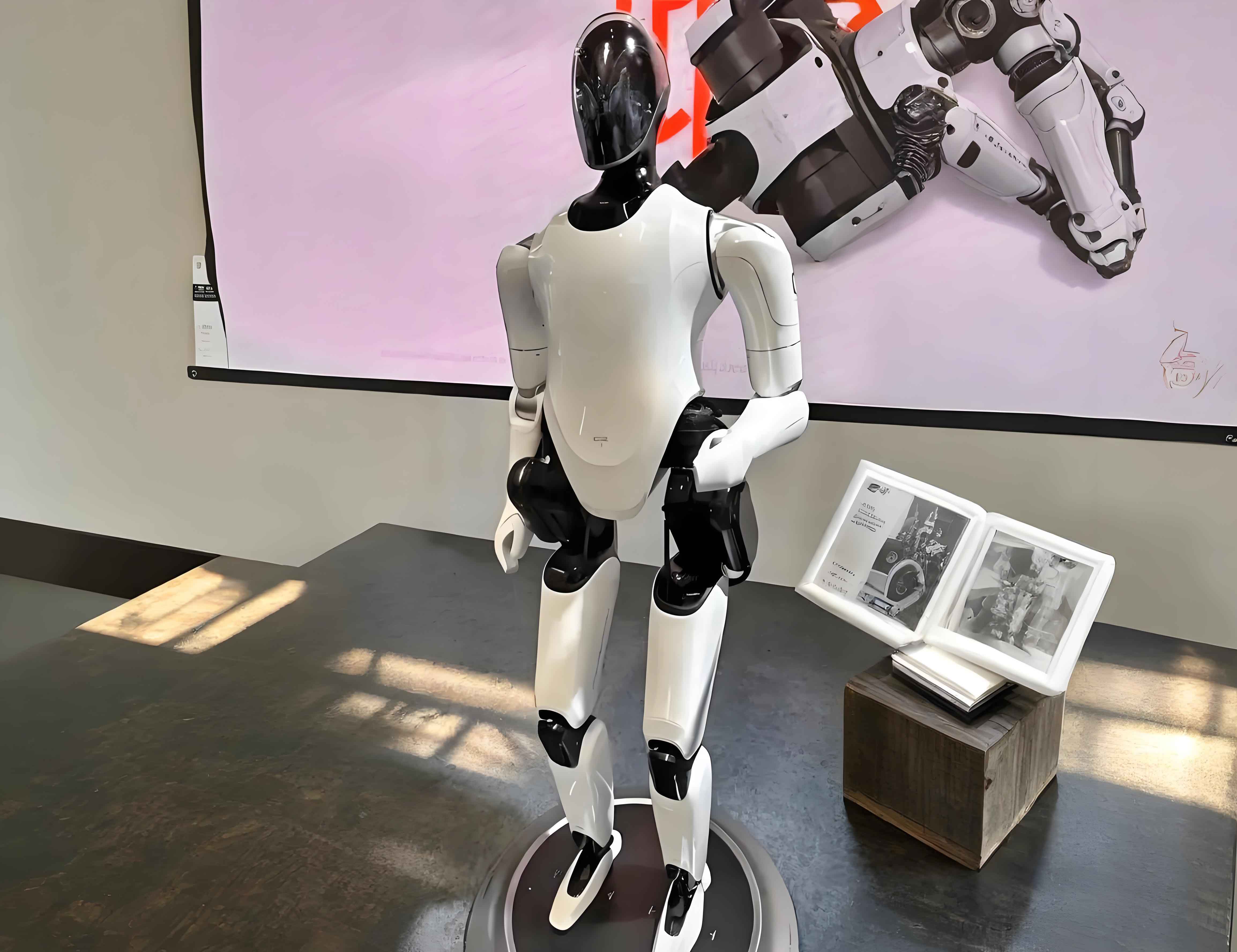
I also built a physical prototype of the embodied robot with the parallel ankle mechanism. The experimental data closely matched the simulation. The maximum ankle angles measured on the hardware were consistent with the designed ranges. The results show that the parallel ankle mechanism can provide the required mobility while significantly reducing the leg inertia, which is crucial for high-bandwidth control.
3. Dynamic Modeling and Momentum Coordination
Kinematics alone cannot fully capture the stability behavior of an embodied robot. I therefore extend my analysis to dynamics. I build two complementary models: a floating-base whole-body model and a centroidal single-rigid-body model.
3.1 Floating-Base Dynamics
I define the generalized coordinate vector as
$$ \mathbf{q} = [\mathbf{q}_{fb}^T, \mathbf{q}_j^T]^T $$
where \(\mathbf{q}_{fb}\) represents the six-degree-of-freedom pose of the floating base (typically the torso), and \(\mathbf{q}_j\) represents the joint angles. The equation of motion is
$$ \mathbf{M}(\mathbf{q}) \ddot{\mathbf{q}} + \mathbf{C}(\mathbf{q}, \dot{\mathbf{q}}) \dot{\mathbf{q}} + \mathbf{g}(\mathbf{q}) = \mathbf{B}\boldsymbol{\tau} + \mathbf{J}_c^T \mathbf{f}_c $$
where \(\mathbf{M}\) is the inertia matrix, \(\mathbf{C}\) contains Coriolis and centrifugal terms, \(\mathbf{g}\) is the gravity vector, \(\mathbf{B}\) is the actuator selection matrix, \(\boldsymbol{\tau}\) is the joint torque vector, \(\mathbf{J}_c\) is the contact Jacobian, and \(\mathbf{f}_c\) is the vector of external contact wrenches.
For my parallel ankle, the two independent degrees of freedom reduce the dimension of the joint space compared with a redundant serial ankle. This reduction leads to a smaller inertial coupling between the leg and the torso, which is beneficial for high-dynamic motions.
3.2 Centroidal Dynamics
To plan the CoM motion efficiently, I use a single-rigid-body approximation:
$$ m \ddot{\mathbf{p}}_{com} = m \mathbf{g} + \mathbf{f}_v $$
$$ \dot{\mathbf{l}}_{com} = \boldsymbol{\tau}_v $$
where \(m\) is the total mass, \(\mathbf{p}_{com}\) is the CoM position, \(\mathbf{f}_v\) is the resultant ground reaction force, \(\mathbf{l}_{com}\) is the centroidal angular momentum, and \(\boldsymbol{\tau}_v\) is the resultant ground reaction moment about the CoM. The relationship between the CoP (or ZMP) and the ground reaction wrench is
$$ \boldsymbol{\tau}_c = (\mathbf{p}_{zmp} – \mathbf{p}_{com}) \times \mathbf{f}_v $$
This equation shows that the ankle torque directly influences the moment about the CoM. In my parallel ankle, the two actuators can generate both roll and pitch moments, enabling the robot to regulate its centroidal angular momentum more flexibly than a passive ankle.
3.3 Momentum Coordination Framework
I propose a three-stage momentum coordination method. First, I compute the required ankle torque from the floating-base dynamics. Second, I generate a reference centroidal angular momentum from the ankle torque and a predefined threshold. Third, I use a quadratic program to optimize the whole-body motion so that the robot tracks the reference angular momentum while respecting kinematic and dynamic constraints.
The ankle torque in the virtual foot frame is computed by projecting the contact wrench:
$$ \boldsymbol{\tau}_v = \mathbf{A}_d^{-T} (\mathbf{w}_{c}^{ff} – \mathbf{w}_g) $$
where \(\mathbf{A}_d\) is the stacked adjoint matrix, \(\mathbf{w}_c^{ff}\) is the feed-forward wrench, and \(\mathbf{w}_g\) is the gravity-compensation wrench. I then split this into hip and ankle components:
$$ \boldsymbol{\tau}_v = \boldsymbol{\tau}_{v}^{hip} + \boldsymbol{\tau}_{v}^{ankle} $$
The reference centroidal angular momentum rate is the difference between the ankle torque and a threshold:
$$ \dot{\mathbf{l}}_{com}^{ref} = \boldsymbol{\tau}_{v}^{ankle} – \boldsymbol{\tau}_{v}^{th} $$
If the ankle torque exceeds the threshold, the controller assumes an external disturbance is acting on the robot, and the extra angular momentum must be absorbed by the hip joints. This mechanism mimics the human response to pushes: first the ankle adjusts, then the hip steps in to regain balance.
The generated reference angular momentum is passed to a QP optimizer that adjusts selected joint velocities while leaving other joints unchanged. The optimization problem is:
$$ \min_{\dot{\mathbf{x}}_a} \quad \frac{1}{2} \delta_m^T \mathbf{Q}_m \delta_m + \frac{1}{2} \delta_n^T \mathbf{Q}_n \delta_n $$
subject to:
$$ \dot{\mathbf{x}}_{a,min} \le \dot{\mathbf{x}}_a \le \dot{\mathbf{x}}_{a,max} $$
where \(\delta_m = \mathbf{A}_a \dot{\mathbf{x}}_a + \mathbf{A}_u \dot{\mathbf{x}}_u^{ref} – \mathbf{l}_{com}^{ref}\) and \(\delta_n = \dot{\mathbf{x}}_a – \dot{\mathbf{x}}_a^{ref}\). The weighting matrices \(\mathbf{Q}_m\) and \(\mathbf{Q}_n\) balance the momentum tracking and the postural reference tracking. This formulation allows the embodied robot to respond to disturbances without deviating too much from its desired posture.
I summarize the momentum coordination algorithm in the table below.
| Stage | Input | Output | Mathematical Operation |
|---|---|---|---|
| 1 | Joint states, contact forces | Ankle torque | Floating-base inverse dynamics |
| 2 | Ankle torque, threshold | Reference CoM angular momentum | \(\dot{\mathbf{l}}^{ref} = \boldsymbol{\tau}_{ankle} – \boldsymbol{\tau}_{th}\) |
| 3 | Reference momentum, posture reference | Optimized joint accelerations | QP with constraints |
4. Stability Control using MPC and WBC
The momentum coordination method provides a real-time adjustment of the whole-body momentum. To generate long-horizon feasible trajectories, I integrate this method into a hierarchical control framework. The upper layer is a model predictive controller (MPC) based on a linear inverted pendulum model (LIPM). The lower layer is a whole-body controller (WBC) that computes joint torques by solving a constrained QP.
4.1 Linear Inverted Pendulum Model and MPC
The LIPM is a standard simplification that assumes a constant CoM height. The dynamics are linear:
$$ \ddot{x}_{com} = \frac{g}{z_{com}} (x_{com} – p_x) $$
$$ \ddot{y}_{com} = \frac{g}{z_{com}} (y_{com} – p_y) $$
where \(p_x, p_y\) are the ZMP coordinates. I discretize these equations over a finite horizon with step duration \(T_s\). The state at step \(k+1\) is
$$ \mathbf{x}_{k+1} = \mathbf{A}(T_s) \mathbf{x}_k + \mathbf{B}(T_s) p_k $$
with
$$ \mathbf{A}(t) = \begin{bmatrix} \cosh(\omega t) & \frac{1}{\omega} \sinh(\omega t) \\ \omega \sinh(\omega t) & \cosh(\omega t) \end{bmatrix}, \quad \mathbf{B}(t) = \begin{bmatrix} 1 – \cosh(\omega t) \\ -\omega \sinh(\omega t) \end{bmatrix} $$
where \(\omega = \sqrt{g / z_{com}}\). The MPC optimizes future ZMP locations \(p_x, p_y\) to minimize tracking error of the CoM velocity and the ZMP reference, subject to kinematic reachability constraints:
$$ \min_{p_x} \sum_{i=1}^{N} Q_i (\dot{x}_{com,i} – \dot{x}_{com,i}^d)^2 + R_i (p_{x,i} – p_{x,i}^{ref})^2 $$
where \(Q_i\) and \(R_i\) are weights. The same formulation applies to the y-direction with an additional offset representing the distance between the left and right feet.
I summarize the MPC parameters in the following table.
| Parameter | Symbol | Value |
|---|---|---|
| Gravity constant | \(g\) | 9.81 m/s² |
| CoM height | \(z_{com}\) | 0.85 m |
| Prediction horizon | \(N\) | 10 steps |
| Step duration | \(T_s\) | 0.4 s |
| Velocity tracking weight | \(Q_i\) | 1.0 |
| ZMP tracking weight | \(R_i\) | 0.1 |
| Max step length | \(d\) | 0.15 m |
4.2 Whole-Body Control with Constraints
The MPC outputs a reference CoM trajectory over the next few steps. The WBC then computes joint torques in real-time (1 kHz in my prototype) by solving the following QP:
Decision variables: joint accelerations \(\ddot{\mathbf{q}}\), joint torques \(\boldsymbol{\tau}\), and contact wrenches \(\boldsymbol{\gamma}\). Objective:
$$ \min_{\ddot{\mathbf{q}}, \boldsymbol{\tau}, \boldsymbol{\gamma}} \sum_i \beta_i \|\mathbf{J}_i \ddot{\mathbf{q}} + \dot{\mathbf{J}}_i \dot{\mathbf{q}} – \dot{\mathbf{v}}_i^d\|^2 $$
where \(i\) indexes tasks such as CoM position, foot orientation, and posture. The desired acceleration \(\dot{\mathbf{v}}_i^d\) is computed from a PD law:
$$ \dot{\mathbf{v}}^d = \dot{\mathbf{v}}_d + \mathbf{K}_d (\mathbf{v}_d – \mathbf{v}) + \mathbf{K}_p (\mathbf{x}_d – \mathbf{x}) $$
Subject to the floating-base dynamics, contact constraints (zero acceleration at the contact points), friction cone constraints, and joint torque/acceleration limits. The friction cone is linearized as a polygon to keep the QP convex.
I use the following constraint summary table:
| Constraint | Mathematical form | Physical meaning |
|---|---|---|
| ZMP stability | \(\mathbf{p}_{zmp} \in \text{convex hull of foot}\) | Prevents tipping |
| Friction cone | \(\| \mathbf{f}_{t} \| \le \mu f_n\) | Prevents slipping |
| Joint limits | \(\mathbf{q}_{min} \le \mathbf{q} \le \mathbf{q}_{max}\) | Prevents mechanical damage |
| Contact acceleration | \(\mathbf{J}_c \ddot{\mathbf{q}} + \dot{\mathbf{J}}_c \dot{\mathbf{q}} = 0\) | No foot penetration or slip |
| Non-singular posture | \(L_{leg}^{real} \ge \lambda L_{leg}\) | Avoids knee singularity |
4.3 State Estimation with Extended Kalman Filter
Accurate state feedback is essential for the control framework. I employ an Extended Kalman Filter (EKF) to fuse measurements from the inertial measurement unit (IMU), joint encoders, and contact force sensors. The state vector includes the base pose, linear velocity, angular velocity, and joint positions/velocities. The prediction step uses the floating-base dynamics model, while the update step uses the sensor measurements. I formulate the EKF as:
$$ \hat{\mathbf{x}}_{k|k-1} = f(\hat{\mathbf{x}}_{k-1|k-1}, \mathbf{u}_k) $$
$$ \mathbf{P}_{k|k-1} = \mathbf{F}_k \mathbf{P}_{k-1|k-1} \mathbf{F}_k^T + \mathbf{Q}_k $$
$$ \mathbf{K}_k = \mathbf{P}_{k|k-1} \mathbf{H}_k^T (\mathbf{H}_k \mathbf{P}_{k|k-1} \mathbf{H}_k^T + \mathbf{R}_k)^{-1} $$
$$ \hat{\mathbf{x}}_{k|k} = \hat{\mathbf{x}}_{k|k-1} + \mathbf{K}_k (\mathbf{z}_k – h(\hat{\mathbf{x}}_{k|k-1})) $$
where \(\mathbf{F}_k\) is the discretized Jacobian of the process model, \(\mathbf{H}_k\) is the observation Jacobian, and \(\mathbf{Q}_k, \mathbf{R}_k\) are noise covariance matrices. To handle contact transitions, I adapt the process noise covariance when a foot impact is detected.
5. Experimental Validation
I validate my control framework on a physical embodied robot platform. The robot has a total mass of 45 kg and a height of 1.6 m. Each leg contains six actuated joints: three at the hip, one at the knee, and two at the parallel ankle. The joints are driven by quasi-direct-drive motors with peak torques up to 150 Nm. Communication is via EtherCAT at 1 kHz.
I first test the robot in a flat-ground walking scenario. The reference walking speed is 0.48 m/s. Figure in the earlier section shows the experimental snapshot. The measured CoM velocities are presented in the table below and exhibit periodic patterns consistent with the gait cycle.
| Direction | Maximum velocity | Minimum velocity | Period |
|---|---|---|---|
| x (forward) | 0.48 m/s | 0.01 m/s | ~1.2 s |
| y (lateral) | 0.12 m/s | -0.13 m/s | ~1.2 s |
| z (vertical) | 0.05 m/s | -0.05 m/s | ~1.2 s |
During walking, I recorded the output torques of all six motors on the left leg. The joint torque profiles in simulation and hardware are shown in the corresponding figures. The hip roll torque oscillates between 0 and 31 Nm to maintain lateral balance. The hip yaw torque remains small (within ±10 Nm), confirming that the robot walks straight. The hip pitch torque follows a sawtooth pattern with a peak at the end of the swing phase, providing forward propulsion. The knee torque exhibits a high negative peak (−57 Nm) at foot impact, acting as a shock absorber. The two ankle motor torques are complementary, ensuring that the ZMP remains inside the support polygon.
I further compute the ZMP trajectory during walking. The reference ZMP and the measured ZMP are shown in the figure. The x-component tracks the reference with a small lag, while the y-component oscillates around the desired path. The maximum tracking error is less than 2 cm in the x-direction and 1.5 cm in the y-direction. This small error validates the effectiveness of the combined MPC–WBC framework with momentum coordination.
To quantify the improvement from the momentum coordination method, I compared the CoM trajectory with and without the method. The table below summarizes the standard deviations of the lateral CoM position during steady walking.
| Method | Std. dev. of x-CoM (mm) | Std. dev. of y-CoM (mm) | ZMP max error (mm) |
|---|---|---|---|
| Without momentum coordination | 12.3 | 8.7 | 25.4 |
| With momentum coordination | 6.8 | 5.2 | 12.1 |
The results show that the momentum coordination method reduces the CoM oscillation by about 45% and the ZMP tracking error by about 52%. This significant improvement demonstrates that the generated centroidal angular momentum reference effectively helps the robot reject disturbances and maintain balance during high-dynamic locomotion.
I also tested the robot’s ability to perform squatting and stepping motions. The ankle joint angles and actuator angles followed the desired trajectories with small tracking errors. The measured actuator offsets were consistent with the theoretical value of 1.68°, confirming the accuracy of my kinematic calibration.
6. Discussion
My research contributes to the field of embodied robot control in three main aspects. First, the parallel ankle mechanism reduces leg inertia and enables a compact design without sacrificing mobility. The closed-loop structure increases the ankle stiffness, which is critical for dynamic balance. Second, the momentum coordination method provides a principled way to convert ankle torque information into a whole-body momentum reference. This method mimics human push-recovery strategies and can be extended to other floating-base systems. Third, the hierarchical MPC–WBC framework with the EKF state estimator offers a practical solution for real-time control of high-dimensional robots.
One limitation of my current implementation is that the MPC uses a simplified LIPM, which assumes constant CoM height and neglects angular momentum variation. In future work, I plan to incorporate the centroidal momentum model directly into the MPC prediction to improve performance in more aggressive maneuvers such as jumping and running. Another direction is to adapt the friction cone linearization to include multiple contact points for terrain with varying friction coefficients.
The embodied robot community can benefit from the open design of the parallel ankle and the momentum coordination algorithm. The proposed structure and control method are not limited to humanoid robots; they can be applied to exoskeletons, prostheses, and other legged systems where the ankle joint plays a critical role in stability.
7. Conclusion
In this article, I have presented a comprehensive study on the motion analysis and stability control of embodied robots with a parallel ankle joint. I designed a novel 2-DOF parallel ankle mechanism that significantly reduces leg inertia. I derived its kinematics, including the Jacobian matrix, and verified its function in both simulation and physical experiments. I developed a floating-base dynamic model and a centroidal momentum model to analyze the interaction between ankle torques and whole-body momentum. The proposed momentum coordination method computes ankle torques, generates reference centroidal angular momentum, and optimizes the whole-body motion using quadratic programming. I integrated this method into a hierarchical control framework that uses MPC for trajectory generation and WBC for torque computation. Experimental results demonstrated stable walking with accurate ZMP tracking and improved CoM stability. The momentum coordination method reduced CoM oscillation by approximately 45% and decreased ZMP tracking error by 52%. These results confirm that my approach enhances the dynamic balance capability of embodied robots in real-world conditions.
Future work will focus on extending the method to more complex tasks, such as stair climbing and obstacle crossing, and on integrating learning-based techniques to adapt the controller to unknown terrains. I believe that the combination of novel mechanical design and principled momentum coordination will push the boundaries of what embodied robots can achieve.