
The quest for agile and robust legged locomotion has been a central focus in robotics research. Among various platforms, the quadruped robot, often colloquially referred to as a robot dog, presents a compelling compromise between stability and mobility. It is capable of executing a variety of gaits, from the statically stable crawl to the dynamic trot and gallop. The jumping gait, characterized by brief aerial phases and high instantaneous ground reaction forces, represents a pinnacle of dynamic performance, enabling the robot dog to traverse gaps or obstacles. However, this gait introduces significant control challenges due to its inherent underactuation during flight phases and the need for precise, high-bandwidth force control during the short contact periods.
Model Predictive Control (MPC) has emerged as a powerful framework for managing such complex, constrained dynamical systems. By leveraging an internal model to predict future system behavior over a finite horizon and optimizing control inputs accordingly, MPC is well-suited for handling the multi-contact dynamics of a legged robot. Nevertheless, a critical bottleneck exists: the computational burden of solving the online optimization problem for a high-degree-of-freedom full-body model often limits the achievable control frequency. This low update rate can hinder the controller’s ability to reject fast disturbances and manage the rapid dynamics of a jump. To address this, I propose a control strategy centered on a simplified robot model that enables high-frequency MPC, specifically tailored for the jumping gait of a parallel-structured quadruped robot, effectively creating a more responsive and stable robot dog.
The core idea is to reduce the computational complexity by exploiting the symmetry and primary dynamics of the jumping gait. When the robot dog executes a bound or a pronk—where the two front legs and the two hind legs move in pairs—its motion is predominantly confined to the sagittal plane. This observation allows for a drastic simplification: the complex quadrupedal system can be modeled as an equivalent planar bipedal robot. In this simplified model, the entire mass of the robot dog is concentrated at its torso center of mass (CoM), and the massless legs act as force actuators at the contact points. This reduction is valid, particularly for parallel-structured designs where the leg mass is often a small fraction (<10%) of the total body mass. The state and control vectors for this simplified model are significantly lower-dimensional than the full-body model, as summarized in Table 1.
| Model Type | State Dimension | Control Input Dimension | Primary Dynamics |
|---|---|---|---|
| Full-Body Robot Dog Model | 12 (position, orientation, & velocities) | 12 (joint torques or spatial forces) | Full 3D multi-rigid-body |
| Simplified Planar Biped Model | 7 (x, ẋ, y, ẏ, θ, θ̇, -g) | 4 (Fxf, Fyf, Fxh, Fyh) | Sagittal plane CoM & pitch |
The dynamics of this planar biped model, representing the core locomotion of the robot dog, are derived in the world coordinate frame. Let $m$ and $I$ denote the total mass and pitch-axis moment of inertia of the robot body. The coordinates $(x, y)$ and angle $\theta$ represent the CoM position and body pitch, respectively. The forces $F_f^x, F_f^y$ and $F_h^x, F_h^y$ are the horizontal and vertical ground reaction forces at the virtual front and hind leg contact points. The vectors $(r_{xf}, r_{yf})$ and $(r_{xh}, r_{yh})$ define the positions from the CoM to the front and hind contact points in the body frame. The equations of motion are:
$$
\begin{align}
m\ddot{x} &= F_f^x + F_h^x \\
m\ddot{y} &= F_f^y + F_h^y – mg \\
I\ddot{\theta} &= F_f^x r_{yf} + F_h^x r_{yh} + F_f^y r_{xf} – F_h^y r_{xh}
\end{align}
$$
By augmenting the state vector to include the gravitational constant $-g$ as a state with zero derivative, the system can be written in the linear state-space form $\dot{\mathbf{X}} = \mathbf{A}\mathbf{X} + \mathbf{B}\mathbf{U}$, where $\mathbf{X} = [x, \dot{x}, y, \dot{y}, \theta, \dot{\theta}, -g]^T$ and $\mathbf{U} = [F_f^x, F_f^y, F_h^x, F_h^y]^T$. This formulation is crucial as it provides a linear prediction model for the MPC.
The high-level MPC controller operates on this simplified model. Its objective is to compute the optimal ground reaction forces $\mathbf{U}$ that drive the robot dog’s CoM state $\mathbf{X}$ to track a desired reference trajectory $\mathbf{X}_{ref}$, which typically includes a constant desired forward velocity and a fixed body height and pitch. The continuous-time model is discretized using a forward Euler method with a time step $T_s$:
$$ \mathbf{X}(k+1) = \bar{\mathbf{A}}\mathbf{X}(k) + \bar{\mathbf{B}}(k)\mathbf{U}(k) $$
where $\bar{\mathbf{A}} = \mathbf{I} + T_s\mathbf{A}$ and $\bar{\mathbf{B}} = T_s\mathbf{B}(k)$. Over a prediction horizon of $N$ steps, the future states are stacked into a vector $\bar{\mathbf{X}}(k)$ and expressed in terms of the current state and a sequence of future controls $\bar{\mathbf{U}}(k)$:
$$ \bar{\mathbf{X}}(k) = \mathbf{\Psi}(k)\mathbf{X}(k) + \mathbf{\Lambda}(k)\bar{\mathbf{U}}(k) $$
The MPC solver then minimizes a quadratic cost function:
$$ J(k) = (\bar{\mathbf{X}}(k) – \bar{\mathbf{X}}_{ref}(k))^T \mathbf{Q} (\bar{\mathbf{X}}(k) – \bar{\mathbf{X}}_{ref}(k)) + \bar{\mathbf{U}}^T(k) \mathbf{R} \bar{\mathbf{U}}(k) $$
subject to practical constraints that reflect the physical limits of the robot dog:
$$ \begin{align}
F_{min} &\leq F^y \leq F_{max} \quad \text{(Leg force capacity)} \\
-\mu F^y &\leq F^x \leq \mu F^y \quad \text{(Friction cone)}
\end{align} $$
Here, $\mathbf{Q}$ and $\mathbf{R}$ are weight matrices, and $\mu$ is the ground friction coefficient. Solving this Quadratic Programming (QP) problem at each control step yields the optimal force sequence, and only the first step $\mathbf{U}(k|k)$ is applied. The simplified model’s low dimensionality allows this QP to be solved at a very high frequency (targeting 500 Hz), enabling reactive control for the dynamic robot dog.
The forces $\mathbf{U}(k|k) = [F_f^x, F_f^y, F_h^x, F_h^y]^T$ computed by the MPC are aggregate forces for the front and hind pairs. To implement this on the actual quadruped robot dog, these forces must be distributed to the four individual legs: Front-Left (FL), Front-Right (FR), Hind-Left (HL), Hind-Right (HR). A simple distribution would be to split them equally. However, to maintain stability in the roll and yaw axes—which are ignored in the planar model—a corrective mechanism is introduced. Proportional-Derivative (PD) controllers are used to generate distribution adjustments $dF_{roll}$ and $dF_{yaw}$ based on the errors in body roll and yaw angles/rates. The final force commands for each leg are:
$$
\begin{align}
F_{FL}^x &= F_f^x / 2 – dF_{yaw}, \quad &F_{FL}^y &= F_f^y / 2 – dF_{roll} \\
F_{FR}^x &= F_f^x / 2 + dF_{yaw}, \quad &F_{FR}^y &= F_f^y / 2 + dF_{roll} \\
F_{HL}^x &= F_h^x / 2 – dF_{yaw}, \quad &F_{HL}^y &= F_h^y / 2 – dF_{roll} \\
F_{HR}^x &= F_h^x / 2 + dF_{yaw}, \quad &F_{HR}^y &= F_h^y / 2 + dF_{roll}
\end{align}
$$
These desired Cartesian forces at each foot must be converted into joint torques. This requires the leg Jacobian matrix $\mathbf{J}_i$, derived from the inverse kinematics of the parallel leg mechanism. If $\boldsymbol{\alpha}_i = [\alpha_{1,i}, \alpha_{2,i}]^T$ represents the joint angles for leg $i$, and $\mathbf{p}_i^b = [x_i^b, y_i^b]^T$ is the foot position in the body frame, the joint torques $\boldsymbol{\tau}_i$ are computed as:
$$ \boldsymbol{\tau}_i = \mathbf{J}_i^T \cdot \mathbf{F}_i^b, \quad \text{where} \quad \mathbf{J}_i = \frac{\partial \mathbf{p}_i^b}{\partial \boldsymbol{\alpha}_i} $$
The body-frame force $\mathbf{F}_i^b$ is obtained from the world-frame force $\mathbf{F}_i$ via a rotation by the body pitch angle $\theta$: $\mathbf{F}_i^b = \mathbf{R}_z^T(\theta) \mathbf{F}_i$. These torques are then commanded to the actuators in the robot dog’s legs.
For the swing phase during the jumping gait, a separate trajectory-tracking controller is used. The foot trajectory for a swinging leg is planned using an 11th-order Bézier curve, $B(t) = \sum_{i=0}^{11} \binom{11}{i} P_i (1-t)^{11-i} t^i$, where $t \in [0,1]$ is the normalized swing phase time and $P_i$ are control points. This ensures a smooth lift-off, transit, and touch-down motion. A critical aspect for gait transition is detecting ground contact. When a leg is in the swing phase, a “virtual force” can be estimated from the joint torques using the same Jacobian transpose relationship: $\mathbf{F}_{virt} = (\mathbf{J}^T)^{\dagger} \boldsymbol{\tau}$. By comparing the measured vertical component of this virtual force to a known baseline (measured when the leg is truly unloaded in the air), a reliable touchdown event can be detected, signaling the transition from swing to stance control for that leg of the robot dog.
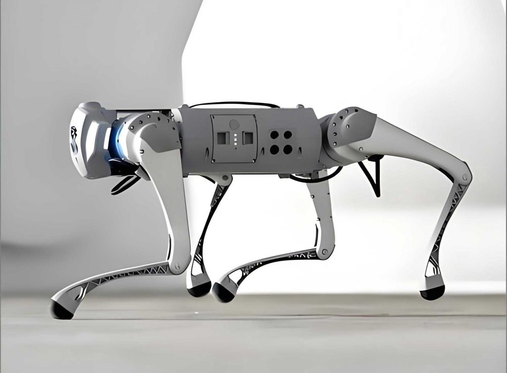
To validate the proposed high-frequency MPC strategy, I developed a prototype parallel-structured quadruped robot dog. The key physical parameters of the platform are listed in Table 2.
| Parameter | Value / Specification |
|---|---|
| Body Dimensions | 430 mm × 280 mm × 60 mm |
| Upper / Lower Leg Length | 92 mm / 220 mm |
| Total Mass | 13 kg |
| Actuator Type | TMotor AK80-6 (12 N·m max) |
| IMU (Orientation) | Yesense YIS100 |
| Control Computer | Onboard Intel NUC |
The experimental goal was to compare the performance of the proposed simplified-model high-frequency MPC (HF-MPC, ~500 Hz) against a traditional full-body model low-frequency MPC (LF-MPC, ~100 Hz) for the jumping gait. The robot dog was commanded to accelerate from rest to and maintain various target speeds (0.5 m/s, 1.0 m/s, 1.5 m/s). The tracking performance for the highest speed (1.5 m/s) is summarized in Table 3, highlighting the advantages of the high-frequency approach.
| Performance Metric | High-Freq MPC (~500 Hz) | Low-Freq MPC (~100 Hz) |
|---|---|---|
| Max Speed Tracking Error | < 0.2 m/s | Up to 0.46 m/s |
| Max Position Tracking Error | ~0.1 m | ~0.23 m |
| Ground Reaction Force Profile | Smooth, lower peak forces (e.g., Fx~14N, Fy~90N) | Jerky, higher peak forces (e.g., Fx~22N, Fy~120N) |
| Controller Behavior | Proactive, fine-grained adjustments | Reactive, coarser corrections |
The experimental data clearly demonstrates the superiority of the HF-MPC strategy. The velocity and position tracking were significantly more accurate and stable. More importantly, the ground reaction forces computed by the 500 Hz controller were smoother and had lower peak magnitudes. This is because the high update rate allows the controller for the robot dog to make proactive, fine-grained adjustments to the forces, preventing the large error accumulation that leads to the jerky, high-peak forces observed with the 100 Hz controller. The smooth force profile is directly linked to stable and efficient locomotion, reducing mechanical stress and energy loss. Additional tests on slopes of 4° and 8° confirmed that the control framework maintains functionality and stability on moderate uneven terrain, demonstrating its robustness for the robot dog platform.
In conclusion, this work successfully addresses the computational bottleneck in applying MPC to dynamic legged gaits. By strategically simplifying the complex model of a quadruped robot dog to an equivalent planar biped model for the jumping gait, I enabled a model predictive controller to run at a very high frequency of approximately 500 Hz. This high-frequency MPC, combined with a PD-based force distribution layer and a separate swing leg controller, provides precise and reactive whole-body control. The experimental validation on a physical parallel-structured robot dog prototype confirms that this approach yields superior tracking performance and smoother, more stable force profiles compared to a conventional low-frequency MPC based on a full-order model. The research demonstrates a practical and effective pathway to enhancing the dynamic performance and stability of agile robot dogs, particularly for challenging gaits like the jump. Future work will focus on extending this simplified-model MPC approach to other dynamic gaits and further improving terrain adaptability.